From HiPPO to H3
Equipping State Space Models for Language
Introduction
The recently-introduced H3 (Hungry Hungry HiPPOs)

In this post, we will explore the motivation behind H3 and the techniques that led to its development, including the Structured State Space Sequence(S4) model
State Space Models
H3 and S4 come from the world of state space models (SSMs), which have a long history in control theory and signal processing. SSMs encode input-output relationships as dynamical systems with some visible and some internal, or hidden, states. The system’s hidden state \(X\) evolves over time according to the differential equation shown below, and the output \(y\) is a function of the current state and the input \(u\). We can write a general SSM as follows:
\[\begin{align*} X'(t) &= A(t)X(t) + B(t)u(t) \\ y(t) &= C(t)X(t) + D(t)u(t) \end{align*}\]It’s fine for our purposes to assume that \(A(t), B(t), C(t), D(t)\) are linear; for any given \(t\), they may be expressed as matrix multiplications. We call systems like this linear state space models. Many SSMs are constructed such that \(A(t), B(t),C(t), D(t)\) do not depend on \(t\) and as such are called time-invariant
Discrete SSMs
In practice, we often work with discrete-time SSMs, in which the state evolves according to recurrence relation like the one below:
\[\begin{align*} Xt &= AX_{t-1} + Bu_t\\ yt &= CX_t+ Du_t \end{align*}\]These discrete steps may correspond to a uniform grid in time, but we can also (i) directly encode the time between observations in the input \(u\), or (ii) use a variable sampling rate, in which case the lengths of each time step can be learned by the model. A variable or adaptive sampling rate could be useful in a number of scenarios:
- When some features of the input are more frequently sampled than others (e.g. a GPS signal that is sampled at 1 Hz and an accelerometer that is sampled at 100 Hz).
- When downstream tasks may require different sampling rates / timescales
Example: Kalman filter
Perhaps the most ubiquitous example of a state space model is the Kalman filter. It is modeled as a discrete state space recurrence with the addition of noise terms \(w_t\) and \(v_t\):
\[X_t = AX_{t-1} + Bu_t + w_t y_t = CX_t + Du_t + v_t\]Let’s unpack this a bit:
- \(w_t\) is the process noise, which represents the uncertainty in the state transition. trajectory. This reflects how well/poorly the dynamics of the system are specified by the linear model.
- \(v_t\) is the measurement noise, which represents the uncertainty in the measurement. Notably, a better measurement tool (e.g. a graduated cylinder instead of a measuring cup) can reduce this noise source, but not the process noise \(w_t\).
This model excels in particular at filtering out the measurement noise \(v_t\), which is why it is so popular in signal processing and mechanical control systems. In these settings, work is often done to characterize the noise sources and to tune the model accordingly.
The Kalman filter has some desirable properties, including:
- A simple derivation for its update rule, which makes it easy to understand and implement.
- A closed-form solution for the posterior distribution of the state given the observations as well as a constant-time update rule
- If its assumptions hold, i.e. the system is correctly specified by the model and the covariance matrices are known, the Kalman filter is minimizes the mean squared error of the state estimate.
The Kalman filter also has some limitations. For nonlinear systems, the Extended Kalman Filter and Unscented Kalman Filter are popular extensions. There is also a growing body of work on the use of Kalman filters in deep learning
Deep SSMs
Despite a number of desirable properties that made them historically successsful, many SSMs are poorly suited to deep learning. This may owe itself to any number of reasons, including:
- Contemporary hardware works more easily with parallelizable operations, and the natural interpretation of an SSM is sequential.
- Although some instances of SSMs can be very efficient and information rich, the general case, in which the transition matrices \(A, B, C\) and \(D\) are arbitrarily initialized and learned, is not.
- State space models require careful initialization and tuning of hyperparameters,and they are not easily interpretable.
With this in mind, there appears to be a need for a new class of SSMs that are more amenable to deep learning. Ideally, these models would:
- Perform well even with irregularly sampled data or unequal timescales
- Be easy to initialize and train
- Exhibit fast inference and training times
- Come with theoretical guarantees and empirical evidence of their performance
And so, we arrive at HiPPO.
HiPPO: High-order Polynomial Projection Operators
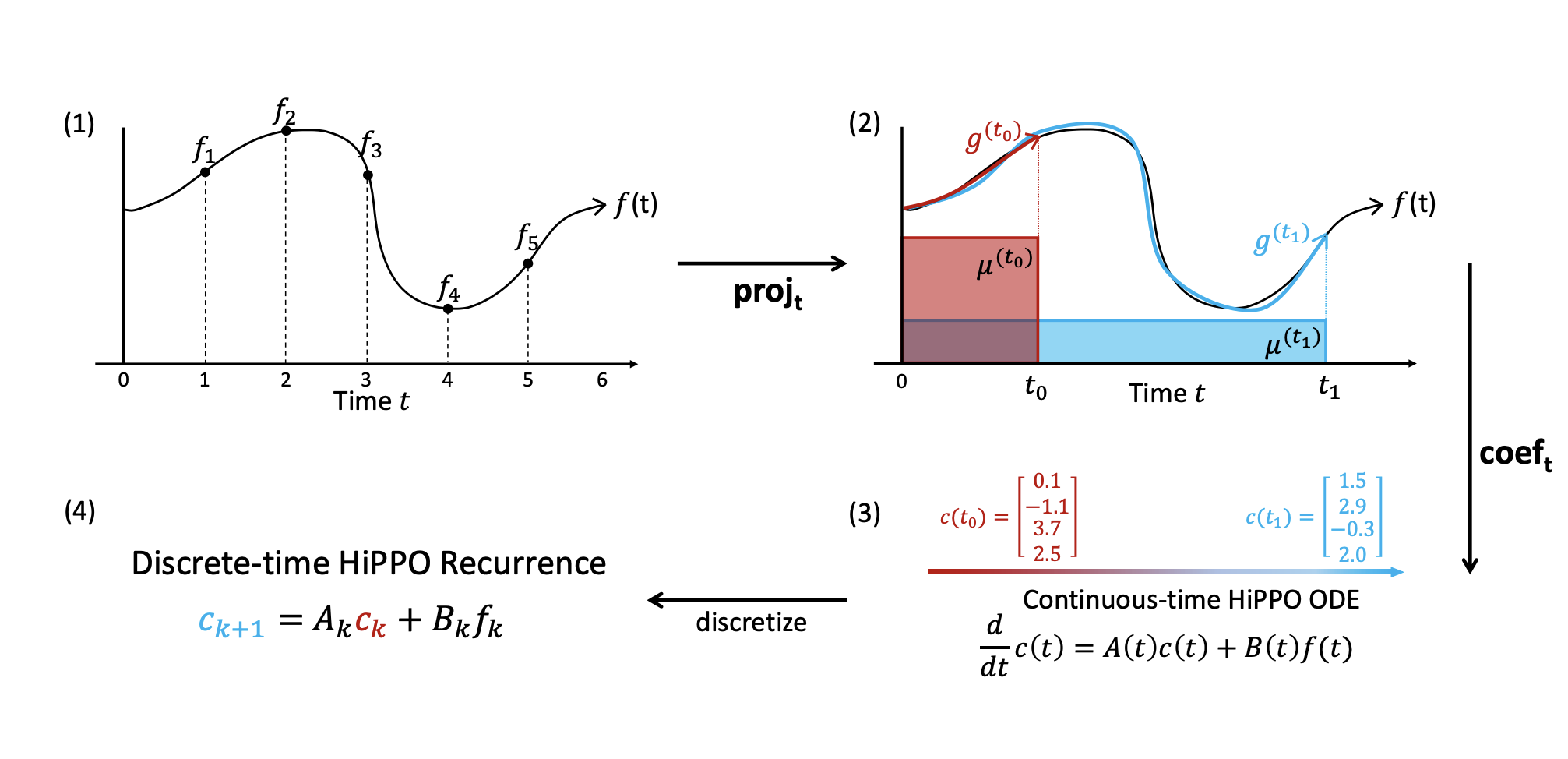
So HiPPO is introduced to address these concerns with deep state space models. How does it work? Well, Let’s jump right into the original definition:
Definition 1. Given a time-varying measure family \(\mu^{(t)}\) supported on \(\\(-\infty, t \\]\), an N-dimensional subspace \(G\) of polynomials, and a continuous function \(f:R≥0→R\), HiPPO defines a projection operator \(proj_t\) and a coefficient extraction operator \(coef\), at every time \(t\), with the following properties:
- \(proj_t\) takes the function \(f\) restricted up to time \(t\) ,\(f≤t:= f(x)\rvert_t\), and maps it to a polynomial \(g(t)\in G\), that minimizes the approximation error \(\lVert f≤t− g(t)\rVert _{L2((t))}\)
- \(coef_t: G → RN\) maps the polynomial \(g(t)\) to the coefficients \(c(t)\) RN of the basis of orthogonal polynomials defined with respect to the measure \(\mu^{(t)\)
Let’s work through the ideas in this definition:
- For a function \(f(t)\) , define \(f_t := f\) restricted to the interval \((-\infty, t]\) . For example, below we have \(f_0 ... f_5\).
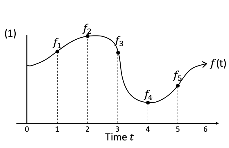
For each t, our goal is to approximate ft using a simple and expressive functional form.
To do this, we need to select a method for describing the approximation error between two given functions. We will do so using a family of measures \(\mu_t\)) that evolve with t. Then, we must select a candidate subspace \(G\subset F\) from which to search for the function \(g(t)\) that minimizes the approximation error between \(f(t)\) and \(g(t)\). We will choose GF to be a space of polynomial functions, and we will express each g(t)G according to a chosen basis of orthogonal polynomials L = (l1 ,l2, … , lN).

With this in place, we can define a function c(t) that maps each t to the corresponding coefficients of g(t) with regards to the orthogonal basis \(L=(l_1, l_2, ... , l_p)\) . Then, we can differentiate \(c(t)\) to produce the ordinary differential equation shown below, which captures the way \(c(t)\) evolves through time as determined by \(f(t)\). \(\frac{d}{dt}c(t) = A(t)c(t) + B(t)f(t)\)
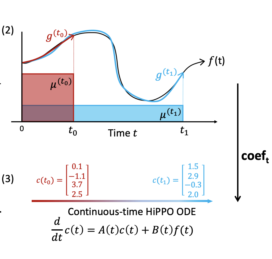
Rather than working with the continous ODE, the authors we will discretize it into a recurrence relation given as
\[c_{k+1} = A_kc_k + B_kf_k\]If we can find operators \(Ak, Bk\) that satisfy the above recurrence, then they satisfy the HiPPO definition and therefore provide the best approximation for the sequence \({fk}\).

Now, let’s apply the HiPPO definition to a specific case. We will see how the construction of a HiPPO operator starts with the selection of a measure family \(\mu^{(t)}\) and then proposes a suitable basis of orthogonal polynomials \(L\) to use in the approximation.
HiPPO-LegT (Legendre Time-invariant)
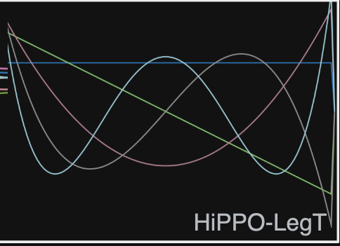
HiPPO-LegT is based on Legendre Polynomials. These are defined as the system of polynomials that satisfy the following:
- They are orthogonal on the interval \([-1, 1]\) with respect to the uniform measure on that interval.
- Denote by \(P_n\) the nth Legendre polynomial. Then, for all \(n\), \(P_n(1) = 1\) and \(P_n(-1) = (-1)^n\).
Gu et al. first consider the Legendre polynomials rescaled and shifted to be orthonormal on the interval \([0, 1]\) with respect to the measure \(\mu^{(t)}(x) = \frac 1 \theta \mathbb I_{\lbrack t-\theta, t\rbrack}\), where \(\theta\) is a constant. In other words, the measure is uniform on the interval \([t-\theta, t]\) and zero elsewhere.
Taking this basis and measure family, the authors show that the discretized ODE for HiPPO-LegT takes the form of a state space model with the following transition matrices:
\(A_{nk} = \frac{1}{\theta}\begin{cases} (-1)^{n-k}(2n+1) & n \geq k \\ 2n+1 & n \leq k \end{cases}\) x \(B_n = \frac 1 \theta (2n+1)(-1)^n\)
In other other words, this just corresponds to a simple sliding window average with equal weights. This naturally motivates the question: what about other types of moving averages? What happens, for example, if we use exponential weighting instead of uniform? But more on that later. First, let’s point out some related work:
The Legendre Memory Unit
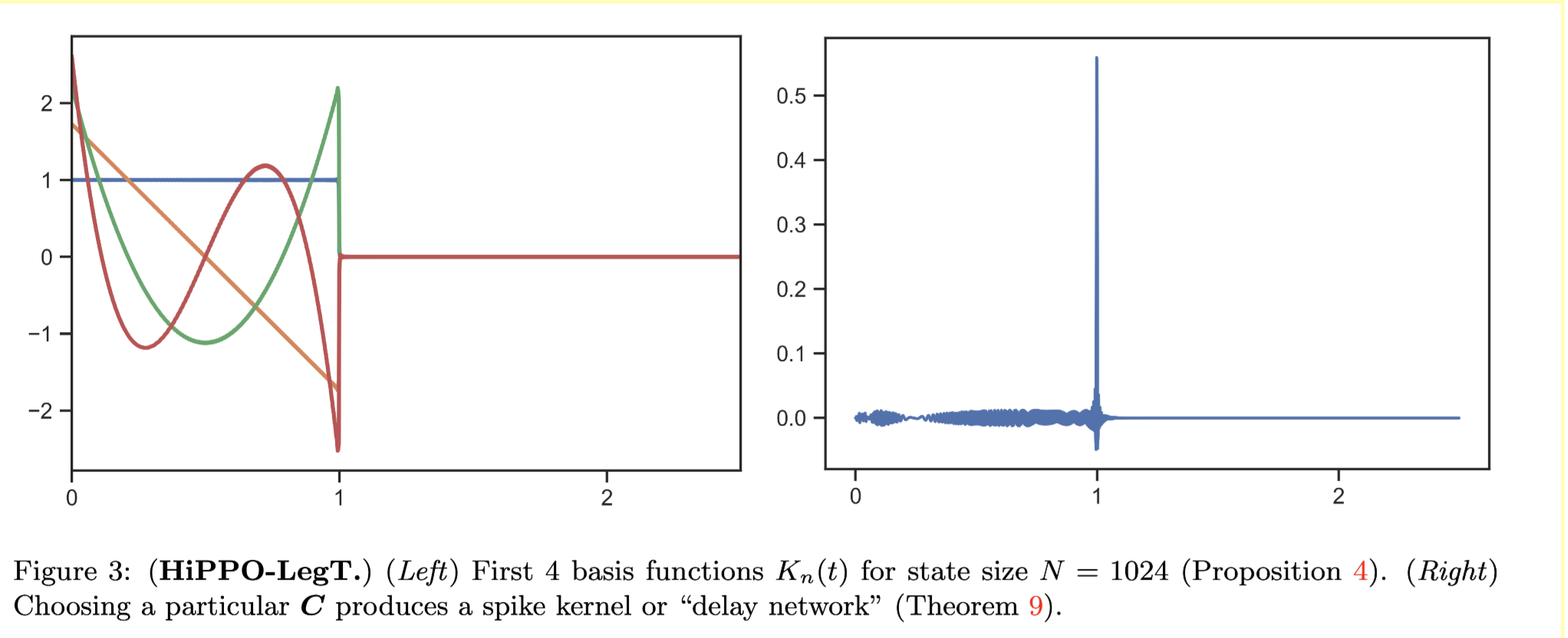
The HiPPO-LegT state space model parameterization is equivalent to that of the Legendre Memory Unit
HiPPO-LagT: Laguerre Time-invariant
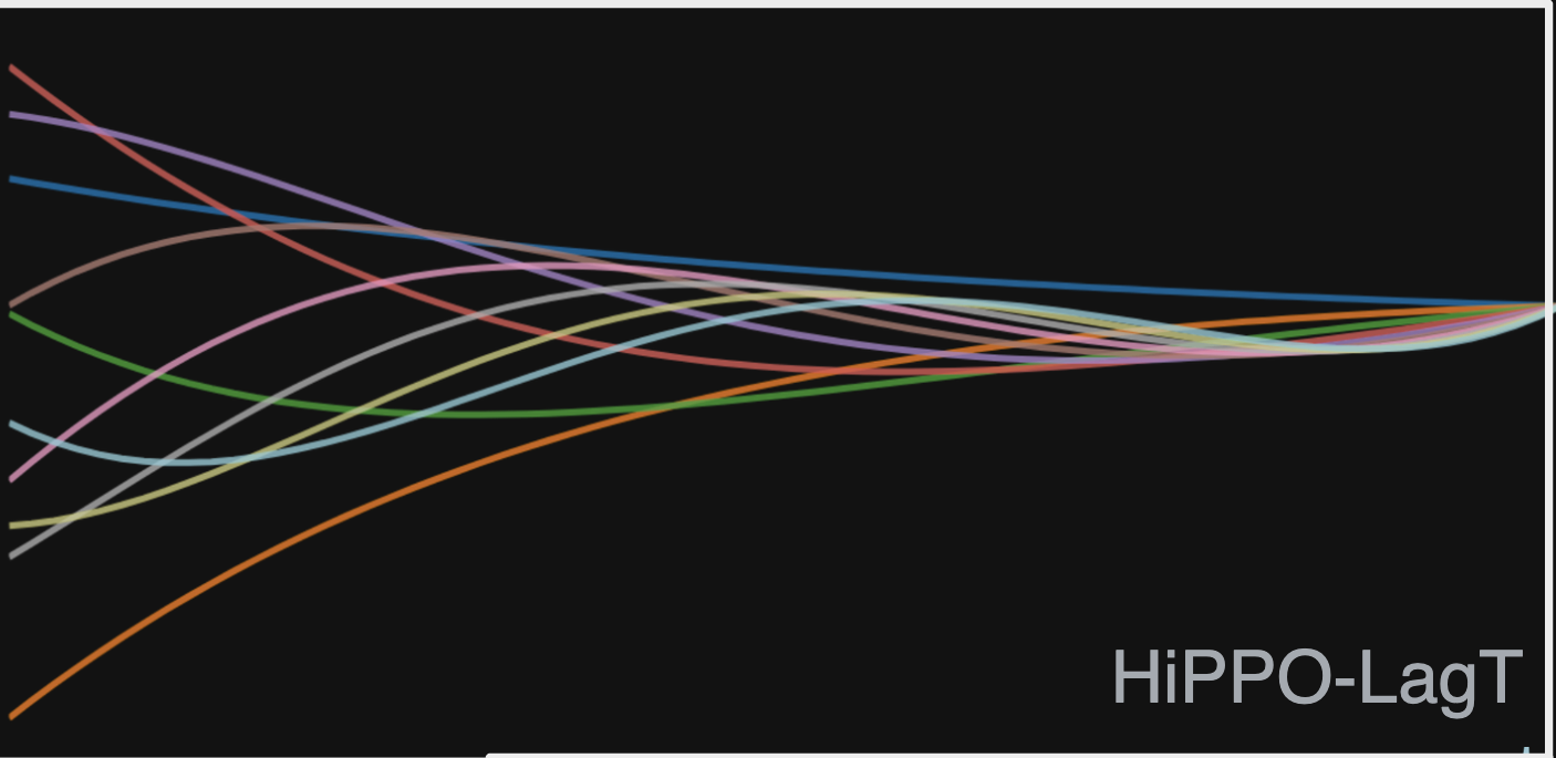
As noted, the HiPPO-LegT model is determined by the choice of a uniform measure that acts like a sliding window average. We can construct the HiPPO operator that corresponds to exponential moving averages as well. In this case, the measure is given by the following:
\[\mu^{(t)}(x) = e ^ {x - t} \mathbb I_{\lbrack -\infty, t\rbrack}(x).\]To find the corresponding state space model, we need to first find a polynomial basis that is orthonormal with respect to this measure. Luckily, this is precisely what the Laguerre polynomials are. The Laguerre polynomials are defined as the system of polynomials that satisfy the following:
- They are orthogonal on the interval \([0, \infty)\) with respect to the measure \(\mu^{(t)}(x) = e ^ {x - t} \mathbb I_{\lbrack -\infty, t\rbrack}(x)\).
- Denote by \(L_n\) the nth Laguerre polynomial. Then, for all \(n\), \(L_n(0) = 1\) and \(L_n'(0) = 0\).
The transition matrices for the HiPPO-LagT state space model are given by:
\[A_{nk} = \begin{cases} 1 & n \geq k \\ 0 & n \leq k \end{cases}\] \[B_n = 1\]HiPPO-LegS: Legendre Scale-invariant
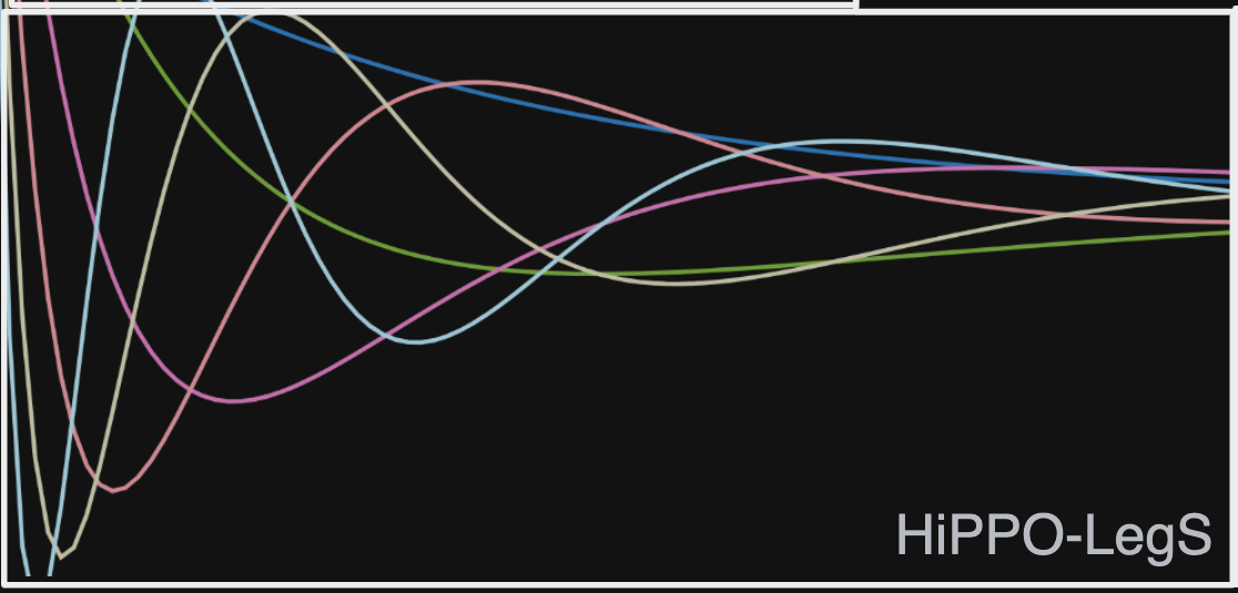
The last two HiPPO variants, HiPPO-LegT and HiPPO-LagT, are both time-invariant, meaning that the transition matrices are the same for all values \(t\). Let’s now consider a scale-invariant variant, HiPPO-LegS.
We start with the scaled Legendre measure (LegS), which assigns uniform weight across an ever-growing interval \([-\infty, t]\). Under this measure, the authors derive the continuous time ODE for HiPPO-LegS, which is given by
\[\frac{d}{dt} c(t) = A(t)c(t) + B(t)f(t)\\ A(t) = \frac 1 t A \\ B(t) = \frac 1 t B\]where \(A\) and \(B\) are the transition matrices for the HiPPO-LegT model. The authors then discretize this ODE to obtain the state space model for HiPPO-LegS. The transition matrices are given by:
\[\begin{align*} A_{nk} &= \begin{cases} (2n+1)^{1/2}(2k+1)^{1/2} & n > k \\ n + 1 & n = k \\ 0 & n < k \end{cases} B_n &= (2n+1)^{1/2} \end{align*}\]Structured State Spaces
While the HiPPO framework the specific HiPPO operators that we’ve discussed so far have proven effective in encoding memory, they are not in general efficient to compute. The “default” view of a discrete state space model is a recurrence relation; each step of the model is computed by multiplying the previous state by the transition matrix.
This, along with the “vanishing gradient” problem, is why RNNs are so slow and difficult to train. Any time we want to compute the state of the model at time \(t\), we have to compute the state at time \(t-1\), \(t-2\), and so on, all the way back to \(t-n\), where \(n\) is the number of steps in the model. And this is something we need to do often during backpropagation!
To remedy this, Gu et al. introduced the Structured State Space Sequence (S4) Model, which uses a special factorization scheme to speed up matrix multiplications without sacrificing expressive power or numerical stability. In fact, because the factorization is so much more efficient, we are able to change the way we view and work with the SSM. Instead of thinking of the model as a recurrence relation that emits a new state and evolves its internal state at each step, we can think of it as a convolution that can be computed across the entire sequence at once. But what do we mean by “structure”?
Structured Matrices
A structured matrix is a matrix than can be multiplied more efficiently than the naive O(n^2) complexity. For example, the fast fourier transform (FFT) can be computed in O(n log n) time because of its structured representation. Similarly, diagonal and block-diagonal matrices are can be multiplied in O(n) time. Matrix structure is a generalization of matrix sparsity to matrices that are not necessarily sparse, but permit efficient multiplication, inversion, and other operations.
Linear Time-invariant SSMs as Convolutions:
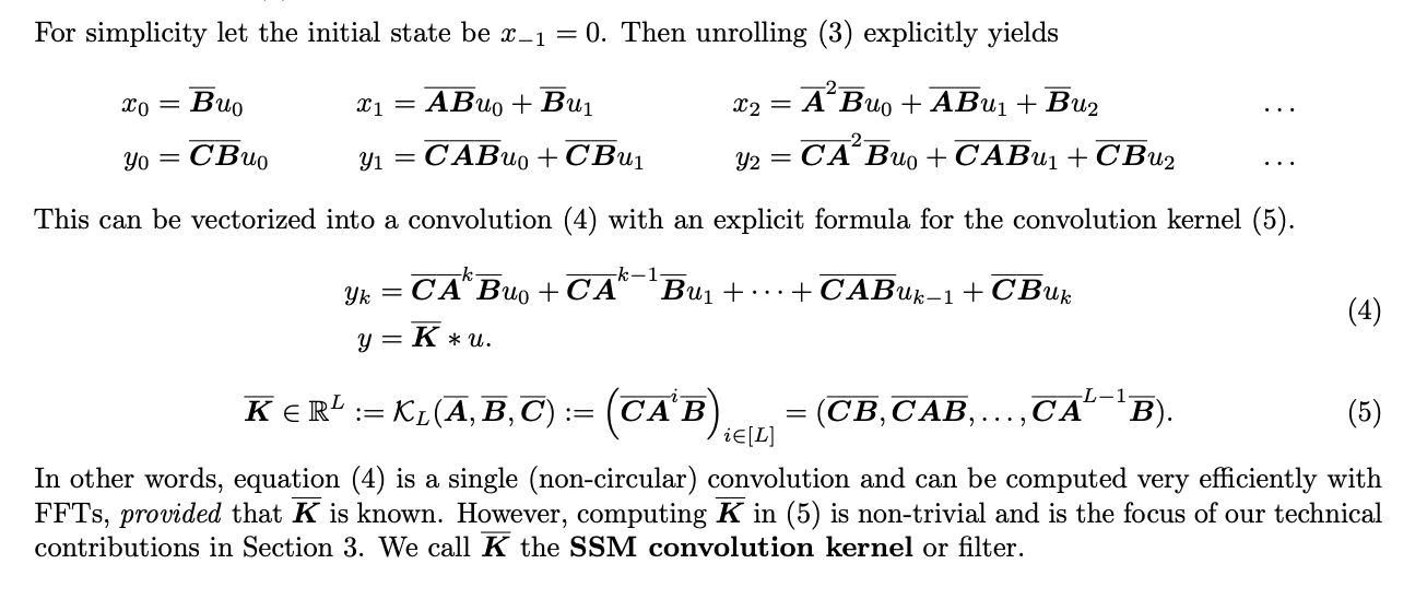
The recurrent form of an arbitrary SSM is poorly suited for training on modern hardware, where parallel computation is the norm. And yet, there is a well-known way to describe a linear recurrence as a convolution: the discrete convolution. The discrete convolution is a linear operation that takes two sequences and produces a third sequence.
The basic idea is that we can “unroll” the recurrence relation into and then refactor it as the convolution of the input sequence with a convolutional kernel \(\bar{K}\). The original authors describe this as follows:

Simple, right?
Normal-plus-low-rank (NPLR) Factorization
Not so simple!
Just because we can write the SSM as a convolution doesn’t mean that we can compute it as a convolution. In fact, the naive implementation of the convolutional kernel is not efficient at all.
The authors of the S4 paper propose using a parameterization called “normal-plus-low-rank” (NPLR). The motivation is simple enough. We know that if the transition matrix \(A\) was diagonal, then we could compute the convolution in \(O((N + L)\log^2(N+L))\) time. Compare this to \((O^2L)\) operations for the naive implementation. This would be all well and good, but we know that the transition matrix is not diagonal.
It turns out, though, that for any of the HiPPO matrices previously discussed, the \(A\) matrix can be written as the sum of a normal matrix and a low-rank matrix. And this gets us much closer to where we need to go.
A normal matrix is a matrix that is the sum of a diagonal matrix and a symmetric matrix. The low-rank matrix is a matrix that can be written as the product of two matrices of lower rank. More explicitly, we have \(A = \Lambda - PP^*\) for some diagonal \(\Lambda \in \mathbb C^{N\times N}\), \(P \in \mathbb C^{N\times r}\), and \(r \ll N\).
Unfortunately, trying to perform the repeated matrix multiplications in the convolution kernel is still not efficient while we have that pesky low-rank term hanging around.
From here, the authors propose and execute a series of clever techniques to get S4 to be more efficient and less prone to divergence. This is, however, our exit ramp for S4. Long live its successor, S4D!
Simplifying S4: Diagonalization
S4D is a diagonal version of S4, and bypasses some of those mind-bending techniques that show up in the implementation of S4.
First the paper recounts the definition of continuous SSMs and their convolutional forms:lg
\[\begin{aligned} \dot{x}(t) &= A(t)x(t) + B(t)u(t) & K(t) &= Ce^{tA}B \\ y(t) &= C(t)x(t) + D(t)u(t) & y(t) &= (K \ast u)(t) \end{aligned}\]We’ve seen the discrete version of this convolution before in the S4 paper, via the construction of the matrix
\[\begin{aligned} \bar{K} = (\bar{C}\bar{B}, \bar{C}\bar{A}\bar{B}, \bar{C}\bar{A^2}\bar{B}, \dots, \bar{C}\bar{A}^{L-1}\bar{B}) = (\bar{C}\bar{A}^i\bar{B})\big|_L \end{aligned}\]We should think of the continous convolution as a linear combination of an infinite number of orthogonal polynomial basis functions. The discrete convolution is a finite approximation of this infinite sum.
The authors of S4D propose a new parameterization for the SSM that is more efficient to compute. The key idea is to diagonalize the transition matrix \(A\), and then use the diagonalization to compute the convolution kernel in the frequency domain.
Some of the big ideas here are:
-
The \(A\) matrix is constrained to have negative eigenvalues,** which keeps the kernel stable. There are multiple ways to enforce this constraint, but the authors do the following: parameterizing \(A\) as \(A = -\exp(A_{Re})+i\cdot A_{Im}\). They also note that any other activation functions bounded on one side could be used in place of \(\exp\) here. They conduct ablation tests with softmax and ReLu, as well as without any activation function at all.
-
The \(B\) vector is frozen at \(B = 1\) for all time. This is because the convolutional term \(\bar K\) relies only on the elementwise product of \(B\) and \(C\) and not the two vectors themselves. In ablations, the authors show that there may be some minor benefit to learning \(B\), but not to any great extent.
-
The SSM parameters \(A, B, C, D\) are now complex-valued, but the input and output, \(u\) and \(y\) respectively, are still real-valued. How did we get here? The authors noted in S4 that complex matrices are, in a sense, more likely to be diagonalizable than real matrices – the set of diagonal matrices is dense in the set of complex matrices. However, because the convolution kernel is conjugate symmetric (it is the same as its complex conjugate), we can use the real-valued form of the Fast Fourier Transform, which is much more efficient to compute. By using the real-valued form of the FFT, we can compute the convolution kernel in \(O(N\log N)\) time, which is much faster than the \(O(N^2)\) time of the naive implementation.
One quick note about complex tensors in deep neural networks: we will soon see that PyTorch has its quirks in working with these data types.
S4D Initializations
The authors share three different initialization schemes for S4D.
-
S4D-LegS: Simply drop the low-rank term of the normal-plus-low-rank factorization of HiPPO-LegS used in S4. Recall the NPLR form was given by \(A = A^{(D)} - PP^T\), with \(A^{(D)}\) being the diagonal matrix containing the eigenvalues of \(A\).
- S4D-Inv: Approximate \(A^{(D)}\) via an empirically determined scaling law. First, we determine that the real component of \(A^{(D)}\) is \(-\frac 1 2 \mathbf 1\), where \(\mathbf 1\) is the matrix of all ones. Next, let \(\mathcal I (A)_n\) denote the n_largest imaginary component in the eigenvalues of \(A^{(D)}\). Then, the authors observe the following:
- \(\mathcal I (A)_0 \rightarrow \frac 1 2 N^2 + c\) for constant \(c \approx 0.5236\).
- All other eigenvalues satisfy an inverse scaling in n: \(\mathcal I (A)_n = \Omega (\frac 1 n)\).
- Simplify the imaginary part of \(A_n\) even further by setting each component to its corresponding Fourier series frequency, i.e. by setting \(\mathcal I (A)_n = i \pi n\) for all \(n\). This is the initialization used in the our implementation below.
S4D Implementation
We’ve already seen how frameworks like HiPPO and models like S4D permit a wide range of possible parameterizations. For the sake of keeping this codebase minimal and easy to understand, we will only implement one specific parameterization of S4D. Our parameterization is based on the following choices:
- Discretization: Zero-order hold (ZOH). The original paper implements ZOH as well as bilinear interpolation.
- Scaling: S4D-Lin.
- Eigenvalue constraint: \(-\exp(A_{Re})\) We constrain \(A\) to have negative real eigenvalues parameterizing it as \(A = -\exp(A_{Re})+i\cdot A_{Im}\).
- Parameterization:
- \(A\): Trainable, complex-valued, real component parametrized as $$\exp(log).
- \(B\): Ones (fixed). Corresponds to the ZOH discretization.
- \(C\): Trainable, complex-valued, normally distributed initial conditions
Alright, let’s get to it. We’ll start with a module that generates the kernel for the S4D layer. We should be able to specify the dimension d_model of each input/output value as well as the dimension d_state of the state matrix. Lastly, we will specify the minimum and maximum time step dt_min and dt_max respectively.
class S4DKernel(nn.Module):
    """Generates a kernel for the S4D layer.

    Args:
        d_model: The number of heads.
        d_state: The dimension of the state matrix
        dt_min: The minimum time step.
        dt_max: The maximum time step.

    Returns:
        A kernel of shape (L, H, N, N)
    """

    def __init__(self, d_model, d_state, dt_min=0.001, dt_max=0.1):
        super().__init__()

        log_dt = torch.linspace(log(dt_min), log(dt_max), d_model)
        log_A_real = torch.log(0.5 * torch.ones(d_model, d_state // 2))
        A_imag = torch.log(0.5 * torch.ones(d_model, d_state // 2))
        C = torch.randn(d_model, d_state // 2, dtype=torch.cfloat)  Complex

        self.log_dt = nn.Parameter(log_dt)
        self.log_A_real = nn.Parameter(log_A_real)
        self.A_imag = nn.Parameter(A_imag)

        # Complex params must be stored as a real tensor of shape (:, 2)
        # or as separate components as we did with A above.
        self.C = nn.Parameter(torch.view_as_real(C))

    def forward(self, L):
        """Generates S4D kernel of shape (L, H, N, N)"""

        # Construct the SSM parameters
        dt = torch.exp(self.log_dt)  # (H)
        A = -torch.exp(self.log_A_real) + 1j * self.A_imag  # (H N)
        C = torch.view_as_complex(self.C)  # (H N)

        # Construct Vandermonde matrix
        dA = A * dt[:, None]
        C = C * (torch.exp(dA) - 1.0) / A
        K = C @ (dA ** torch.arange(L)).T
        return 2 * K.real
There shouldn’t be anything too surprising in this code by now. One quick thing to note is the use of torch.view_as_real and torch.view_as_complex to convert between real and complex tensors. For some reason, PyTorch doesn’t like it if we try to pass a complex tensor as an nn.Parameter.
This kernel is constructed via Vandermonde multiplication. A Vandermonde matrix is one whose columns are powers of a vector. For example, we can construct the Vandermonde matrix of degree \(N\) for a vector \(X\) as \(\begin{align} V^{(N)} &= \begin{bmatrix}X^0 & X^1 & X^2 & ... & X^N\end{bmatrix} \\ & \\ &= \begin{bmatrix} 1 & X_1 & X_1^2 & ... & X_1^N \\ 1 & X_2 & X_2^2 & ... & X_2^N \\ 1 & X_3 & X_3^2 & ... & X_3^N \\ \vdots & \vdots & \vdots & \ddots & \vdots \\ 1 & X_N & X_N^2 & ... & X_N^N \end{bmatrix} \end{align}\)
With the kernel in hand, let’s turn our attention to the S4D layer.
class S4D(nn.Module):
    """S4D (Diagonal Structured State Space Sequence Model) layer.
    Args:
        d_model: The number of heads.
        d_state: The dimension of the state matrix.
        kernel_args: Arguments to pass to the kernel, i.e. only dt_min, dt_max in this implementation.
    """

    def __init__(self, d_model, d_state, **kernel_args):

        super().__init__()
        self.d_model = d_model
        self.d_state = d_state
        self.D = nn.Parameter(torch.randn(d_model))
        self.kernel = S4DKernel(d_model, d_state, **kernel_args)

    def forward(self, u):
        """Input and output shape (B, H, L)"""
        L = u.size(-1)
        kernel = self.kernel(L=L)

        # Perform convolution in the frequency domain
        u_f = rfft(u, n=2 * L) / L
        kernel_f = rfft(kernel, n=2 * L)
        y = irfft(kernel_f * u_f, n=2 * L)

        # Truncate to original length and add skip connection
        y = y[..., :L] + u * self.D[:, None]
        return y
Here we see the S4D layer in action. The input u is a tensor of shape (B, H, L) where B is the batch size, H is the number of heads, and L is the sequence length. The output y is also a tensor of shape (B, H, L). The D parameter is a vector of length H that is used to scale the skip connection.
After computing the kernel, we perform a convolution in the frequency domain. This is done by taking the Fourier transform of the input and kernel, multiplying them, and then taking the inverse Fourier transform. This is a lot faster than computing the convolution in the time domain. We then truncate the output to its original length \(L\) and add the skip connection.
That takes care of all our pre-reqs. Now we can finally implement the H3 layer!
H3: Hungry Hungry HiPPOs

Rather than diving into the H3 paper and working our way down, we’ll start by writing an H3 layer and then working our work our way up. We have an rather simple implementation of H3, so let’s just jump in.
class H3(nn.Module):
    """The Hungry Hungry Hippos (H3) layer.
    Args:
        d_model: The number of heads.
        d_state: The dimension of the state matrix.
        kernel_args: Arguments to pass to the S4D kernel.
    """

    def __init__(self, d_model, d_state=64, **kernel_args):
        super().__init__()
        self.d_model = d_model
        self.d_state = d_state
        self.q_proj = nn.Linear(d_model, d_model)
        self.k_proj = nn.Linear(d_model, d_model)
        self.v_proj = nn.Linear(d_model, d_model)
        self.s4d = S4D(d_model, d_state, **kernel_args)
        self.shift = Shift(d_model, d_state)

    def forward(self, x):
        q = rearrange(self.q_proj(x), "b h l  ->  h l b")
        k = rearrange(self.k_proj(x), "b h l  ->  h l b")
        v = rearrange(self.v_proj(x), "b h l  ->  h l b")
        shift_out = self.shift(k)
        s4d_out = self.s4d(v * shift_out)
        out = rearrange(q * s4d_out, "h l b -> b h l")
        return out
The skeleton of the H3 bears some resemblance to the attention mechanism in the Transformer. In fact, H3 is intentionally designed to resemble the mechanism of linear attention
Self-attention
Self-atention is computed as shown below. For layer input \(X\), the layer projects \(X\) into \(Q, K, V\) matrices. Then, with \(d_k\) as the dimension of the key matrix \(K\), the attention function is defined as follows:
\[\begin{align*} \text{Attention} & = & V'& = \text{softmax}(\frac{QK^T}{\sqrt{d_k}})V \end{align*}\]Linear Attention
Linear attention, introduced by () , is a simple extension of self-attention that aims to draw a throughline between the Transformer and the RNN. To obtain the framework for linear attention, we first rewrite the attention function as follows:
- Start with standard attention: \(V'= \text{softmax}(\frac{QK^T}{\sqrt{d_k}})V\)
- Rewrite in terms of rows/columns instead of matrices: \(V'_i= \frac{\sum_{j=1}^L e^{q^TK}}{\sum_{j=1}^L e^{q^TK}}v_j\)
- Instead of the softmax, we can substitute an arbitrary similarity function sim. So all together we have the following: \(V'_i= \frac{\sum_{j=1}^L sim(QK)}{\sum_{j=1}^L sim(q^TK)}v_j\)]
- Linear attention makes the assumption that the similarity function itself is linear, unlike the softmax, but that it operates on the output of a non-linear kernel \(\phi\) applied to each of \(Q\), \(K\), and \(V\):
The authors then show that this framework connects the Transformer to the RNN. In particular, they show that the output at any given time is a function of two cumulative sums:
- The output \(O_i\) at time \(i\) is given by \(O_i = \frac{\sum_{j=1}^i \phi(K_j)V_j^T}{\sum_{j=1}^i \phi(K_j)}\)
- Let \(S_i = \sum_{j=1}^i \phi(K_j)V_j^T\)
- Let \(z_i = \sum_{j=1}^i \phi(K_j)\)
- Let \(d_i = \phi(Q_i)^Tz_i\)
- Then \(O_i = \frac{\phi(Q_i)^TS_i}{d_i}\)
In other words, the output at time \(i\) is a function of the cumulative sum of the kernel applied to \(K\) and \(V\), and the cumulative sum of the kernel applied to \(Q\). This is exactly the same as the RNN, where the output at time \(i\) is a function of the cumulative sum of the input \(X\) and the cumulative sum of the hidden state \(H\).
This is a very interesting result, and one which motivated the development of H3.
H3
So how does H3 differ from standard and linear attention? First, we have the presence of two state space models within the H3 layer. One of them is a standard S4D or similar SSM, and the other SSM features a specially constructed transition matrix we will call a shift matrix.
The shift SSM’s transition matrix \(A\) has the following basic form:
\[\begin{align*} A_{nk} = \begin{cases} 1 & k = n - 1 \\ 0 & otherwise \end{cases} \end{align*}\]Let’s see what happens when we apply our shift matrix to the state \(X = \begin{pmatrix} x_1 & x_2 & x_3 & x_4 \end{pmatrix}^T\):
\[\begin{align*} Ax &= \begin{pmatrix} 0 & 0 & 0 & 0 \\ 1 & 0 & 0 & 0 \\ 0 & 1 & 0 & 0 \\ 0 & 0 & 1 & 0 \end{pmatrix} \begin{pmatrix} x_1 \\ x_2 \\ x_3 \\ x_4 \end{pmatrix} = \begin{pmatrix} 0 \\ x_1 \\ x_2 \\ x_3 \end{pmatrix} \end{align*}\]So this matrix is shifting the state vector to the right by one. This is exactly what we want, because we want to create interactions between the current token and the previous tokens, and that won’t happen if we only have diagonal transition matrices. Instead, we need to keep the past tokens within reach in some sense, and that’s precisely the role of the shift matrix.
Consider what happens immediately after the shift matrix is applied: we perform an elementwise multiplication between the shifted state and the query vector \(Q\). This is the same as the linear attention mechanism, where we perform an elementwise multiplication between the query and the key. Now, the corresponding elements being multiplied come from different time steps. Again, that’s exactly what we want.
The authors mention that we can let \(B\) be fixed or make it a trainable parameter. In the code, we stick with a fixed value for today. Specifically, the see tht B is set to the matrix consisting of all zeros except for a 1 in the first column. This has the effect of multiplying the first element of the shifted state by the first element of the query, the second element of the shifted state by the second element of the query, and so on. Because this process is ever-repeating, this “shift by one” operation will in fact set up a linear relationship between each token and its entire history.
Let’s see the code:
class Shift(nn.Module):
    """The shift state space layer.
    Args:
        d_model: The number of heads.
        d_state: The dimension of the state matrix.

    The shift layer is a special case of an SSM layer with a fixed A matrix that
    allows tokens to mix with past tokens. For d_state = 4, the A matrix would be:

    A = [[0, 0, 0, 0],
         [1, 0, 0, 0],
         [0, 1, 0, 0],
         [0, 0, 1, 0]]
    """

    def __init__(self, d_model, d_state):
        super().__init__()
        self.d_state = d_state
        self.d_model = d_model
        self.B = torch.zeros(d_model, d_state)
        self.B[..., 0] = 1.0
        self.C = nn.Parameter(torch.randn(1, d_model, d_state))
        self.D = nn.Parameter(torch.randn(d_model))

    def forward(self, u):
        """Input and output shape (B, H, L)"""

        L = u.size(-1)

        # Construct kernel
        B_fc = rfft(self.B, n=2 * L).conj()
        C_f = rfft(self.C, n=2 * L)
        kernel = irfft(B_fc * C_f, n=2 * L)
        kernel = rearrange(kernel[..., :L], "b h l -> b l h")

        # Perform convolution by kernel
        kernel_f = rfft(kernel, n=2 * L)
        u_f = rfft(u, n=2 * L)
        y = irfft(u_f * kernel_f, n=2 * L)

        # Truncate to original length and add skip connection
        y = y[..., :L] + u * self.D[:, None]
        return y
Nothing too interesting here after the last few layer definitions. Lots of convolutions being carried out in the frequency domain, etc.
Well, that’s it for building our model! We’ve covered the basics of H3 and state space models, and we’ve seen how to implement them in PyTorch. Now let’s see how our model does on some toy language tasks from the H3 paper.
Language Tasks
Dao et al introduce two toy language tasks near the beginning of the H3 paper to demonstrate its distinct capabilities compared to more general SSMs. For these tasks, the authors considered toy-scale models of the H3 family, the S4D family, a simple Transformer, and another SSM variant called the gated state space.
First, a base class, then we’ll introduce the fun stuff. Our LanguageTask class is quite simple. It has a few methods that we’ll use to encode tokens into tensors, and decode them back into sequences of tokens. We’ll also define a method to return an embedding layer for the task’s vocabulary,
class LanguageTask:
    """Base class for language tasks.

    Each task should implement the following methods:
        __init__: Initialize the task.
        generate_sequence: Generate a sequence of tokens for the task.
    """

    def generate_sequence(self):
        """This is a method must be implemented by each task."""
        raise NotImplementedError

    def get_embedding_layer(self, embedding_dim):
        """Return an embedding layer for the task vocabulary."""
        return nn.Embedding(len(self.alphabet), embedding_dim)

    def encode_sequence(self, sequence):
        """Convert a sequence of tokens to a tensor of indices."""
        return torch.tensor([self.vocab[token] for token in sequence])

    def decode_sequence(self, sequence):
        sequence = sequence.tolist()
        """Convert a tensor of indices back into a sequence of corresponding tokens."""
        return [self.inv_vocab[token] for token in sequence]
Induction head / copying task
The name “induction head” comes from recent literature in mechanistic interpretability, or the study of how neural networks learn to detect patterns and even execute algorithms via logical and arithmetic circuits.
- Prefix matching: The head attends back to previous tokens that were followed by the current and/or recent tokens.
- Copying: More attention to a token increases the probability that the head will output that token next.
H3 is motivated by the fact that the other SSMs in H3’s family do not exhibit these properties, despite their ability to learn to attend to complex patters over long sequences.
This is clear when we look at the original results.


The toy attention model performs perfectly on both tasks. H3 does perfectly on one task and right under the Attention model on the other. The other SSMs in H3’s family do not perform well at all. They particularly struggle with the copying task, which matches the intuition that they are not able to “log tokens after particular events”.
Alright, on to the tasks. First, the induction head task.
class InductionHeadTask(LanguageTask):
    """Toy language task to test for "copying" capabilities.

    The task is to learn to repeat the token that is shown after the special token '_'.
    We use an alphabet of 19 standard letters, plus the special token.
    The model is trained on sequences of 30 tokens. In each sequence, the pair ('_' + letter) is shown twice,
    and all other tokens are sampled randomly with replacement from the set of standard letters.

    Example sequences:
        'a _ b c a c _ b'
        'b _ a c b c _ a'
    """

    name = "induction_head"
    seq_length = 30
    normal = list("abcdefghijklmnopqrs")
    special = "_"
    alphabet = normal + [special]
    vocab = {token: idx for idx, token in enumerate(alphabet)}
    inv_vocab = {idx: token for token, idx in vocab.items()}

    def generate_sequence(self):
        answer = self.special + np.random.choice(self.normal)
        base = list(np.random.choice(self.normal, self.seq_length - 4, replace=True))
        base = list(np.random.permutation(base + [answer]))
        return list("".join(base + [answer])) # convert to list of chars
For “Induction head”, we task the model with learning to treat a token as a “copying” token. This task has an alphabet of 19 normal characters 'abc..s' and one special character _. The model is trained on sequences of 30 tokens. In each sequence, the pair ('_' + letter) is shown twice, and all other tokens are sampled at random.
To put it differently, in each sequence, we will see the special character “_” twice. The first time, it will be followed by a random letter. The second time, it will be followed by that same letter. The model is tasked with learning to repeat the letter shown earlier in the sequence.
For example, the sequence 'a _ b c a c _ b' is a valid sequence for this task. The model should learn to repeat the letter 'b' after the second _ token. This task sounds simple but it does require sophisticated circuits within the model to learn.
Associative memory task
class AssociativeMemoryTask(LanguageTask):
    """Toy language task for associative memory.

    The task is to learn to associate a key with a value at inference time.
    The model is trained on sequences of key-value pairs, where the keys and values
    are shuffled in each sequence. Each key-value pair is shown twice in each sequence,
    and accuracy is measured only by the final value in the sequence.

    Example sequences:
        'a 1 b 2 c 3 b 2 c 3 a 1'
        'b 3 c 1 c 1 a 2 a 2 b 3'

    Although the example above features 3 keys and values, this task is hard-coded with an alphabet of 10 keys and 10 values,
    as in the original paper.
    """

    name = "associative_memory"
    keys = list("abcdefghij")
    vals = list("0123456789")
    alphabet = keys + vals
    vocab = {token: idx for idx, token in enumerate(keys + vals)}
    inv_vocab = {idx: token for token, idx in vocab.items()}

    def generate_sequence(self):
        shuffled_vals = np.random.permutation(self.vals)
        pairs = list(zip(self.keys, shuffled_vals))
        pairs = np.random.permutation(pairs * 2)
        sequence = [x for pair in pairs for x in pair]
        return sequence
The second task tests “Associative memory”. The model is trained on sequences of key-value pairs, where the keys and values are shuffled in each sequence. Each key-value pair is shown twice in each sequence, and accuracy is measured only by the final value in the sequence.
For example, the sequence 'a 1 b 2 c 3 b 2 c 3 a 1' is a valid sequence for this task. The model should learn to associate the key 'a' with the value '1' and the key 'b' with the value '2'. The model should then be able to correctly predict the value '1' when shown the key 'a' at inference time.
Wrapping up
We’ve just seen how the introduction of a shift SSM made the H3 model more capable at reasoning with text-based tasks and cognitive operations like copying and associative memory. There is still so much to explore in the H3 paper and related works, but I hope this post has given you a taste of the power and expressivity of state space models.
If you’re interested in learning more about state space models, I highly recommend the following resources in addition to cited papers and references.
The codebase for this blog post: The official H3 codebase: https://github.com/hazyresearch/h3 The official S4 codebase: https://github.com/hazyresearch/s4