Rethinking the Implementation Tricks and Monotonicity Constraint in Cooperative Multi-agent Reinforcement Learning

QMIX [8], a very classical multi-agent reinforcement learning (MARL) algorithm, is often considered to be a weak performance baseline due to its representation capability limitations. However, we found that by improving the implementation techniques of QMIX we can enable it to achieve state-of-the-art on the StarCraft Multi-Agent Challenge (SMAC) testbed [10]. Specifically, we evaluated the effect of optimizer, number of rollout processes, replay buffer size, eligibility traces, hidden size and the degree of annealed exploration on QMIX, and tried to explain their role in MARL. Furthermore, the key factor of the monotonicity constraint of QMIX was found in this post, we tried to explain its role and corroborated its superior performance by combining it with another actor-critic style algorithm. We have open-sourced the code at https://github.com/hijkzzz/pymarl2 for researchers to evaluate the effects of these proposed techniques. We hope this research will advance the MARL community and contribute to the establishment of new baselines of QMIX.

Since AlphaZero beats humans at Go, RL has become a consistent hot spot in academia and industry. The agent of RL can obtain some rewards by interacting with the environment and taking actions to maximize these cumulative rewards. Actually, almost all the RL problems can be described as Markov Decision Processes as illustrated in Figure 1.

Figure 1: The agent-environment interaction in a Markov decision process. (Image source: Sec. 3.1 Sutton & Barto (2017) [14])). $R_t, S_t, A_t$ denote the reward, state and action at timestep $t$.

Just as its name implies, MARL contains multiple agents trained by RL algorithms in the same environment. Many complex multi-agent systems such as robot swarm control, autonomous vehicle coordination, and sensor networks, can be modeled as MARL tasks. The interaction of these agents would make them work together to achieve a common goal.

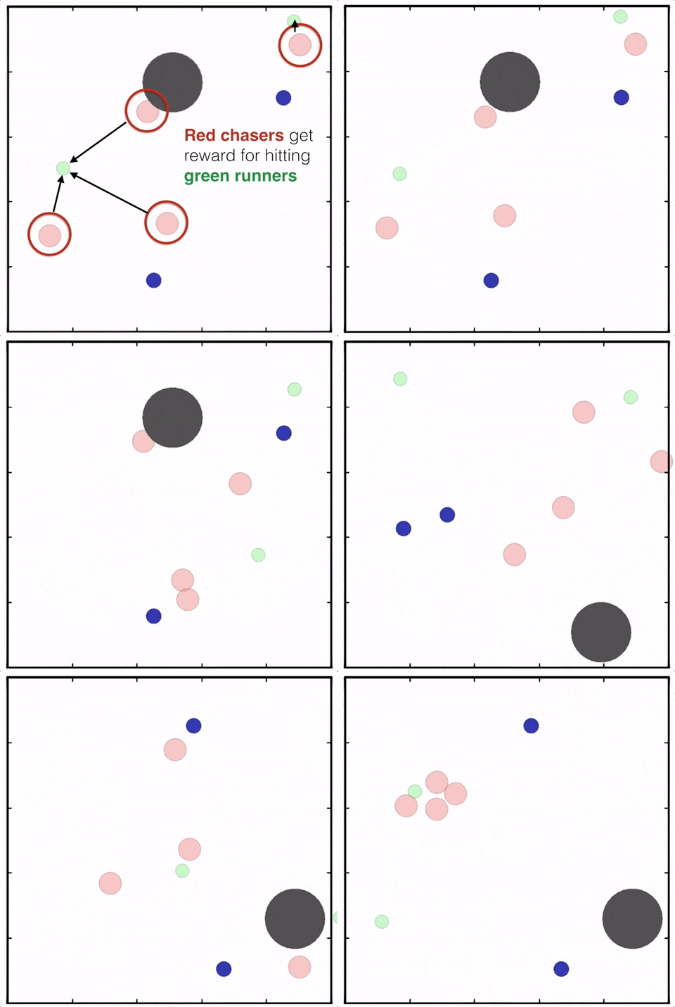
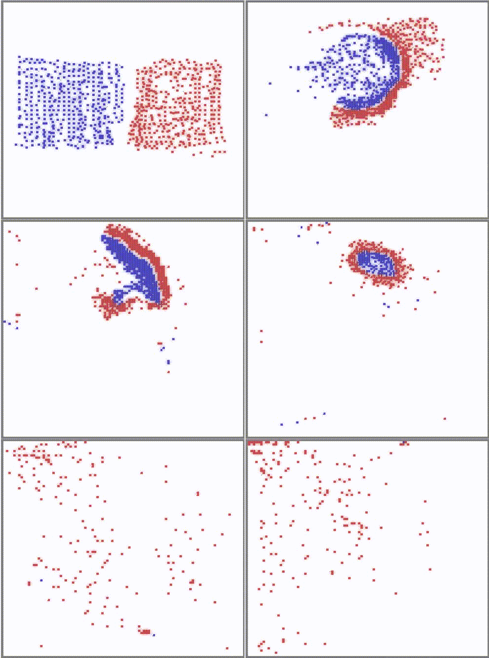
Figure 2: Some multi-agent cooperative scenarios [from-left-to-right].
(a) Chasing in Multi-Agent Particle Environment (Predator-Prey); (b) MAgent Environment;
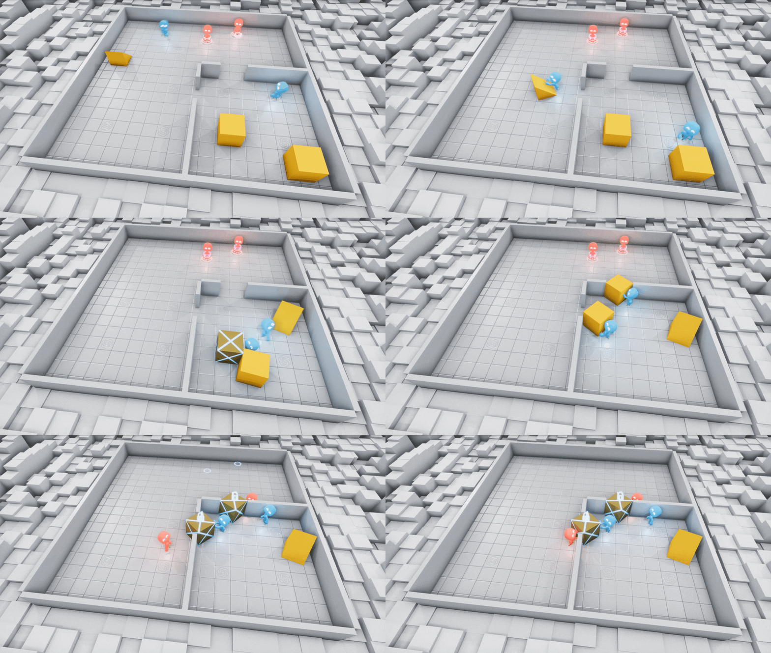
(c) Hide & Seek; (d) StarCraft Multi-Agent Challenge.

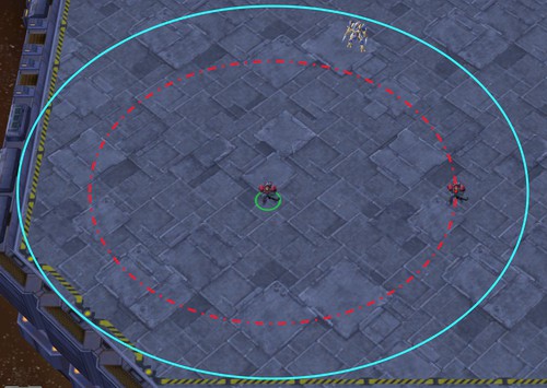
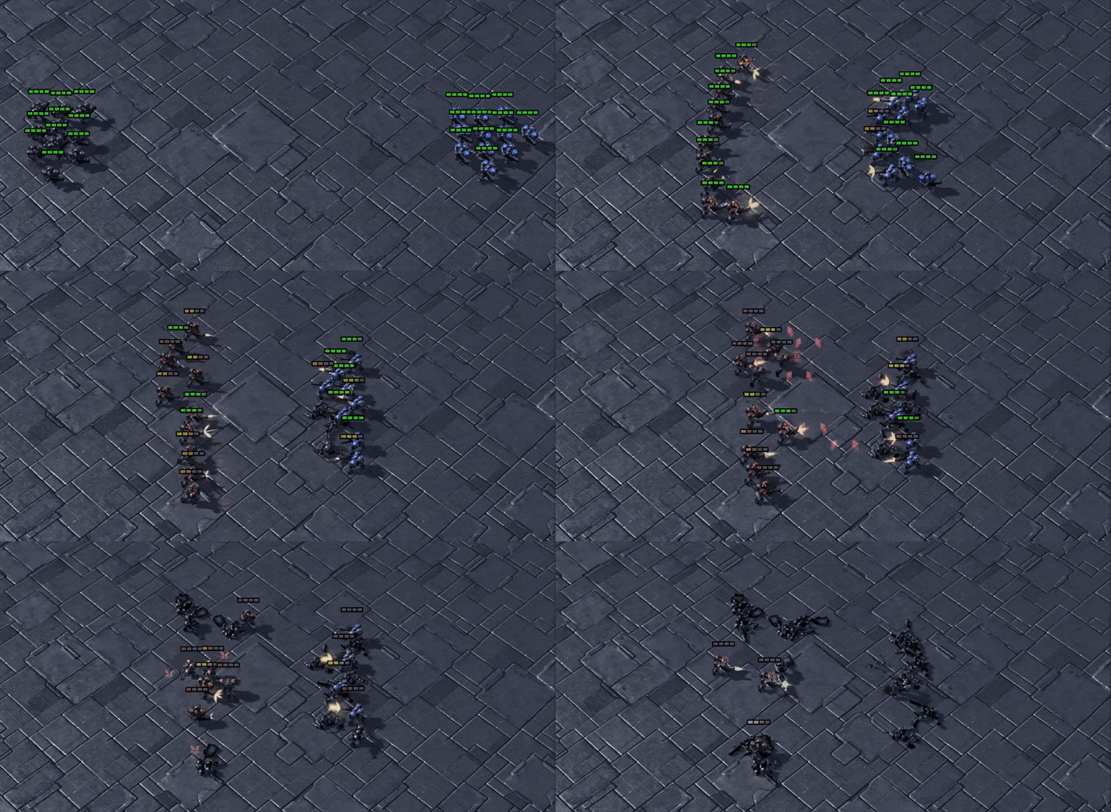
In this general setting, agents usually have a limited sight range to observe their surrounding environment. As shown in Figure 3, the cyan border indicates the sight and shooting range of the agent, which means the agent could only obtain the information of terrain or other agents in that range. This restricted field of view may also result in the difficulty of agents to access to global state information, making its policy updates subject to bias and unsatisfactory performance. In general, these kinds of multi-agent scenarios can be modeled as Decentralized Partially Observable Markov Decision Processes (Dec-POMDP) [6].

Even though many RL algorithms [14] and their variants have been successfully extended to the cooperative scenarios in MARL setting, few of their performance is satisfactory. One of the most troublesome issues is Non-Stationarity. Specifically, as a part of the environment, the changing policies of other agents during training would make the observation non-stationary from the perspective of any individual agent [28] and significantly slow down the policy optimization of MARL. This situation has forced researchers to seek a method that can exploit global information during training but does not destroy the ability of the agents to only use their respective observations during execution, to find a joint policy $\boldsymbol{\pi} = \langle \pi^{1},…,\pi^{n}\rangle$ to maximize global reward. Naturally, the simplicity and effectiveness of the Centralized Training with Decentralized Execution (CTDE) paradigm have attracted the attention of the community, and many MARL algorithms based on CTDE were proposed, making a remarkable contribution to MARL.

In the rest of this section, we briefly introduce Dec-POMDP and CTDE to facilitate the understanding of the contents of MARL, the QMIX algorithm and the following text.

Figure 3: The partial observation of agents
(Image source: SMAC [10]).

Decentralized Partially Observable Markov Decision Process

A Decentralized Partially Observable Markov Decision Process (Dec-POMDP) model, as described in [8][28], is typically used to represent a full cooperative multi-agent task. The model consists of a tuple denoted by $G=(S, U, P, r, Z, O, n, \gamma)$, and involves $n$ agents, where $n$ is an integer between 1 and $n$, inclusive. The true state of the environment, denoted by $s \in S$, describes global information that is relevant to both agents and other auxiliary features. At each timestep $t$, a transition in the environment occurs via a joint action $\mathbf{u} \in \mathbf{U} \equiv U^{n}$, which is composed of an action $u^i \in U$, chosen by each agent. This transition is driven by the state transition function $P\left(s^{\prime} \mid s, \mathbf{u}\right): S \times \mathbf{U} \times S \rightarrow[0,1]$. Additionally, there is a shared global reward function, denoted by $r(s, \mathbf{u}): S \times \mathbf{U} \rightarrow \mathbf{R}$, which is optimized by the whole team. Finally, each agent has a partial observation described by $o^i \in O$, which is derived from the observation function $Z(o^i \mid s, u^i) : S \times U \rightarrow O$. All agents work cooperatively to maximize the shared global reward $R_{t}=\sum_{k=0}^{T} \gamma^{k} r_{t+k}$, which is described by the joint value function $Q^{\boldsymbol{\pi}}\left(s_{t}, \mathbf{u}_{t}\right) = \mathbb{E}_{s_{t+1: \infty}, \mathbf{u}_{t+1: \infty}}\left[R_{t} \mid s_{t}, \mathbf{u}_{t}\right]$.

Centralized Training with Decentralized Execution and Value Decomposition

To better explore the factors affecting the QMIX algorithm, our focus lies in the Centralized Training with Decentralized Execution (CTDE) paradigm of MARL algorithms. These algorithms under this paradigm have access to the true state $s$ and the action-observation histories $\tau^{i}$ of all agents to centrally train policies, but each agent can only rely on its local observation $o^{i}$ for decision-making. Some value-based algorithms implemented under CTDE follow the Individual-Global-Max (IGM) principle [11], ensuring consistency between the joint action-value function $Q_{tot} \left(\boldsymbol{\tau}, \mathbf{u}\right)$ and individual agent-utilities $[Q_i\left(\tau^i, u^i\right)] _{i=1} ^{n}$:

\[\underset{\mathbf{u}}{\operatorname{argmax}}\ Q_{tot} \left(\boldsymbol{\tau}, \mathbf{u}\right) = (\underset{u^{1}}{\operatorname{argmax}}\ Q_{1} \left(\tau^{1}, u^{1}\right), \ldots, \underset{u^{n}}{\operatorname{argmax}}\ Q_{n} \left(\tau^{n} , u^{n}\right)). \tag{1} \label{eq1}\]

One of the most typical ways to efficiently train the joint value function $Q_{tot} \left(\boldsymbol{\tau}, \mathbf{u}\right)$ is to decompose it into the utility functions $[Q_i\left(\tau^i, u^i\right)] _{i=1} ^{n}$ and maintain updating consistency between them via IGM. The simplest factorization structure, called additivity, has been proposed by VDN [13], which makes VDN simply factorize $Q_{tot}$ into a sum of per-agent utilities $Q_{tot}^{\mathrm{VDN}} \left(\boldsymbol{\tau}, \boldsymbol{u}\right)=\sum_{i=1}^{n} Q_{i} \left(\tau^{i}, u^{i}\right)$. VDN’s simplicity and equal weighting of each utility in the joint value function makes it ineffective for cooperative tasks, which has motivated the QMIX structure and other more efficient decomposition approaches.

Notations

In this subsection, we define the notations used in this post. Specifically, in traditional RL, time steps $t$ are usually represented in the update formula and the value function of RL is considered to be estimated by the pairwise variables at the current time step $t$ and the next time step $t+1$. Since the ID of the agent also needs to be represented in the MARL algorithm, it may cause ambiguity when expressed in the same formula as the time step $t$. For simplicity of expression, variables without $t$ are indicated to be implemented at the current time step, while variables at the next time step are indicated with an apostrophe in the upper right corner in the rest of the context, e.g., $s$ means the current state and $s^{\prime}$ indicates the next time step state, the same approach applies to actions $u$ and observations $o$. All the notations are listed in Table 1.

Table 1: All the notations used in this post.

Notation	Description	Notation	Description
$s$	the current state (at time $t$)	$S$	the set of all states
$s^{\prime}$	the next state (at time $t+1$)	$U$	the set of all actions
$u^{i}$	the action of agent $i$	$N$	the set of all agents
$\mathbf{u}$	the joint actions (at time $t$)	$\tau^{i}$	the action-observation history of agent $i$
$o^{i}$	the observation of agent $i$	$${\tau}$$	the joint action-observation histories
$$o$$	the joint observation	$r(s, \mathbf{u})$	the joint reward supplied by environments
$Q_{i}(\tau^{i}, u^{i})$	the utility function of agent $i$	$\gamma$	the discount factor
$Q_{tot}({\tau}, \mathbf{u})$	the joint value function	$P(s^{\prime} \mid s, \mathbf{u})$	the transition function
$Z(o^{i} \mid s, u^{i})$	the observation function	$\epsilon$	action selection probability of $\epsilon$-greedy
$N$	the set of all agents with $n$ agents	$$\theta$$	the set of parameters of agents network, with $[\theta^{i}]_{i=1}^{n}$
$b$	sampled batch size for training	$\phi$	the parameter of mixing network
$TS$	the $T$otal rollout $S$amples	$PP$	the number of rollout $P$rocesses in $P$arallel
$SE$	the number of $S$amples in each $E$pisode	$PI$	the $P$olicy $I$teration number

QMIX and Monotonicity Constraint

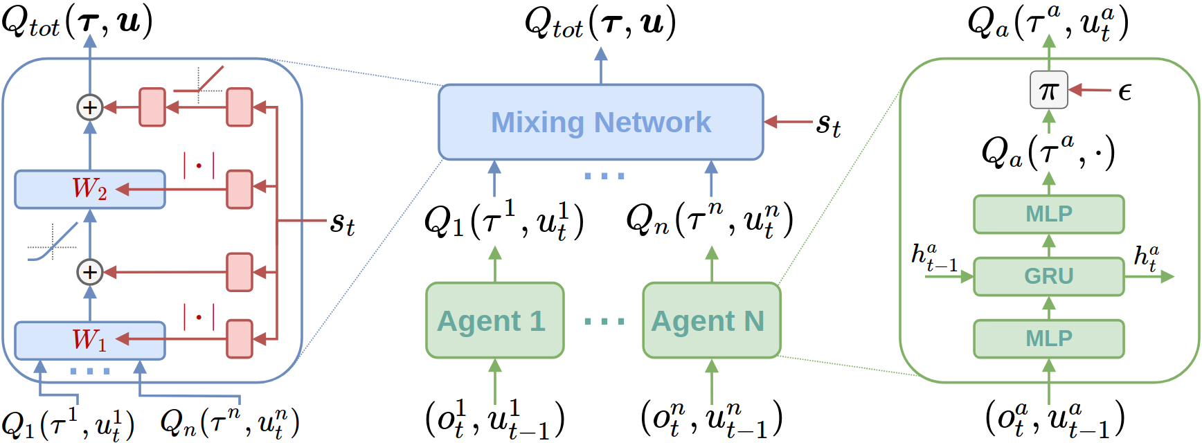
To deal with the relationship between the individual agent and the cooperative group, QMIX [8] learns a joint action-value function $Q_{tot}$ and factorizes the joint policy into the individual policy of each agent. In other words, as illustrated in Figure 4, QMIX integrates all the individual $Q_{i}$ with a mixing network to obtain a centralized value function $Q_{tot}$, which can be more appropriately updated by the global reward.

Figure 4: Framework of QMIX. (Image source: QMIX [8]). On the left is Mixing Network (A Hypernetwork), and on the right is the Agent network.

Still, it also can be represented in Eq.(\ref{eq2})

\[Q_{tot}(s, \boldsymbol{u} ; \boldsymbol{\theta}, \phi) = g_{\phi}\left(s, Q_{1}\left(\tau^{1}, u^{1} ; \theta^{1}\right), \ldots, Q_{n}\left(\tau^{n}, u^{n} ; \theta^{n}\right)\right);\] \[with \quad \frac{\partial Q_{tot}(s, \boldsymbol{u} ; \boldsymbol{\theta}, \phi)}{\partial Q_{i}\left(\tau^{i}, u^{i}; \theta^{i}\right)} \geq 0, \quad \forall i \in N. \tag{2} \label{eq2}\]

where $\theta^i$ is the parameter of the agent network $i$, $u^{i}$ denotes the action of agent $i$, and $\phi$ is the trainable parameter of the mixing network. The the mixing network $g_{\phi}(\cdot)$ is responsible to factorize $Q_{tot}$ to each utility $Q_{i}$. The Monotonicity Constraint is also implemented in the mixing network $g_{\phi}(\cdot)$, which inputs the global state $s$ and outputs non-negative wights through a hyper-network as illustrated in the left part of Figure 4, which will result in $\frac{\partial Q_{tot}(s, \boldsymbol{u} ; \boldsymbol{\theta}, \phi)}{\partial Q_{i}\left(\tau^{i}, u^{i}; \theta^{i}\right)} \geq 0$. This delicate design ensures consistency between joint actions and the individual actions of each agent, then guarantees the Individual-Global-Max (IGM) principle. Benefiting from the monotonicity constraint in Eq. (\ref{eq2}), maximizing joint $Q_{tot}$ is precisely the equivalent of maximizing individual $Q_i$, which would also allow the optimal individual action to maintain consistency with optimal joint action. Furthermore, QMIX learns the centralized value function $Q_{tot}$ by sampling a multitude of transitions from the replay buffer and minimizing the mean squared temporal-difference (TD) error loss:

\[\mathcal{L}(\theta)= \frac{1}{2} \sum_{i=1}^{b}\left[\left(y_{i}^{}-Q_{tot}(s, u ; \theta, \phi)\right)^{2}\right] \tag{3} \label{eq3}\]

where the TD target value $y=r+\gamma \underset{u^{\prime}}{\operatorname{max}} Q_{tot}(s^{\prime},u^{\prime};\theta^{-},\phi^{-})$, and $\theta^{-}, \phi^{-}$ are the target network parameters copied periodically from the current network and kept constant for a number of iterations. $b$ is the sampled training batch size. Due to the strong constraints in Eq.(\ref{eq2}), QMIX is still criticized for the insufficient expressive capacity of the joint value function [3].

Extension to QMIX

Experimental Design

To facilitate the study of proper techniques affecting the training effectiveness and sample efficiency of QMIX, we perform a set of experiments designed to provide insight into some methods that have been proven effective in single-agent RL but may be ambiguous in MARL. In particular, we investigate the effects of Adam optimizer with parallel rollout process; the incremental replay buffer size; the number of parallel rollout processes; $\epsilon$-exploration steps; the implementation of $Q(\lambda)$ in centralized value function; the hidden size of the recurrent network of agents. And we also dive into the role of monotonicity constraints in QMIX. For all experiments, we generally implement PyMARL [10] framework to implement QMIX. To ensure fairness we run independent 3 to 6 experimental trials for each evaluation, each with a random seed. Unless otherwise mentioned, we use default settings as in PyMARL whenever possible, while incorporating the techniques of interest. To prevent the training process of the algorithm from crashing by chance, we remove the highest and lowest scores when counting the calculated returns and win rates for the test episode. All the results are plotted with the median and shaded the interval, and the final scores were not smoothed for the sake of image aesthetics, and we did so to verify exactly what direct effect the proposed techniques could have on QMIX.

StarCraft Multi-Agent Challenge (SMAC) As a commonly used testing environment, SMAC [10] sets an example to offer a great opportunity to tackle the cooperative control problems in the multi-agent domain. We focus on the micromanagement challenge in SMAC, which means each agent is controlled by an independent agency that conditions on a limited observation area, and these groups of units are trained to conquer the enemy consisting of built-in AI. According to the quantity and type of enemy, all testing scenarios could be divided into Easy, Hard, and Super-Hard levels. Since QMIX can effectively solve the Easy tasks, we pay attention to some Hard and Super-Hard scenarios that QMIX failed to win, especially in Corridor, 3s5z_vs_3s6z, and 6h_vs_8z.

Predator-Prey (PP) is representative of another classical problem called relative overgeneralization [16] . The cooperating predators are trained to chase a faster running prey, and hope to capture this escaping robot with the fewest steps possible. We leverage Predator-Prey-2 (a variant of Predator-Prey) proposed in FACMAC [29], whose policy of prey is replaced with a hard-coded heuristic policy. The heuristic policy asks the prey to move to the farthest sampled position to the closest predator. If one of the cooperative agents collides with the prey, a team reward of +10 is emitted; otherwise, no reward is given. In the original simple tag environment, each agent can observe the relative positions of the other two agents, the relative position and velocity of the prey, and the relative positions of the landmarks. This means each agent’s private observation provides an almost complete representation of the true state of the environment.

To introduce partial observability to the environment, the view radius is added to the agent, which restricts the agents from receiving information about other entities (including all landmarks, the other two agents, and the prey) that are out of range. Specifically, we set the view radius such that the agents can only observe other agents roughly 60% of the time. These environments require greater cooperation between agents.

Optimizer

As an important part of training neural networks, the selection of an optimizer is very important since it could seriously affect the training effect of the reinforcement learning agent. Without a further illustration, QMIX uses RMSProp [21] to optimize the neural networks of agents as they prove stable in SMAC. While Adam [1] is famous for the fast convergence benefiting from the momentum in training, which seems to be the first choice for AI researchers. We reckon that the momentum property in Adam would have some advantages in learning the sampled data which is generated by agents interacting with the environment as in MARL. And then, on the other hand, QMIX is criticized for performing sub-optimally and sampling inefficiency when equipped with the A2C framework, which is implemented to promote the training efficiency of the RL algorithm. VMIX [12] argues this limitation is brought about by the value-based inherent Q function, so they extend QMIX to the actor-critic style algorithm to take advantage of the A2C framework. This controversy attracts our attention to evaluate the performance of QMIX using Adam, as well as the parallel sampling paradigm.

Figure 5: The performance of QMIX optimized by Adam and RMSProp.

Results As shown in Figure 5, we run the Adam-supported QMIX with 8 rollout processes. Different from what was described in VMIX, the performance and efficiency of QMIX could be greatly improved by Adam. We speculate the reason is the momentum property in Adam could fastly fit the newly sampled data from the parallel rollout processes and then enhance the performance, while RMSProp failed.

Rollout Process Number

Naturally, we come to focus on the benefits of parallel data sampling in QMIX. A2C [5] provides an excellent example to reduce training time and improve the training efficiency in single-agent RL. As we implement the algorithms under the paradigm of A2C, there is usually a defined total number of samples and an unspecified number of rollout processes. The total number of samples $TS$ can be calculated as $TS = SE \cdot PP \cdot PI$, where $TS$ is the total sum of sampled data, $SE$ denotes the number of samples in each episode, $PP$ and $PI$ denote the number of rollout processes in parallel and the policy iteration number, respectively. This section aims to perform analysis and spur discussion on the impact of the parallel rollout process on the final performance of QMIX.

Figure 6: The performance of different rollout process numbers of QMIX. When given the total number of samples, the performance of fewer processes achieves better performance.

Results Still, we use Adam-supported QMIX to evaluate the effect of the number of the rollout process. Since we could choose the Parallel model to sample the interacting data of the agent with the environment in PyMARL, we can theoretically get more on-policy data which is close to the updating policy in training. Figure 6 shows that when $TS$ and $PP$ is given, the performance enhancement of QMIX is not consistent with the increase in rollout process number. The intuitive explanation is when we set the fewer rollout processes, the greater the quantity of policy would iterate [14]. Besides, too fast updated data in parallel may cause the factitious unstable training in policy updating, i.e., it is difficult for agents to learn effective information from rapidly sampled data from the replay buffer. The more times policies are iterated, the more information the agents would learn which lead to an increase in performance. However, it also causes longer training time and loss of stability. We suggest trying the fewer rollout process in the beginning and then balancing between training time and performance.

Replay Buffer Size

Replay buffer plays an important role in improving sample efficiency in off-policy single-agent RL. Its capacity would greatly affect the performance and stability of algorithms. Researchers usually set a very large capacity of replay buffer in Deep Q-network (DQN) [4] to stabilize the training. Some research on the effect of replay buffer in single-agent RL has already been carried out in [22] , which poses the distribution of sampled training data should be close as possible to the agents’ policies to be updated. Actually, there are two factors affected when we change the capacity of the replay buffer: (1) the replay capacity (total number of transitions/episodes stored in the buffer); and (2) the replay ratio (the number of gradient updates per environment transition/episode) of old policies. When we increase the capacity of the replay buffer, the aged experiences of old policies would grow as the replay ratio is fixed. Then the distribution of outdated experiences would also be much different from the updating policy, which would bring additional difficulty to the training agents. From the results in [22], there seems to be an optimal range of choices between replay buffer size and replay ratio of experiences in RL, where we would like to know whether it is consistent with the results in MARL.

Figure 7: Setting the replay buffer size to 5000 episodes allows for QMIX’s learning to be stable.

Results The results seem not to be consistent with that in single-agent RL. Figure 7 shows the large replay buffer size of QMIX would cause instability during training. When we increase the buffer size from the default setting in PyMARL, the performance would almost continuously declines. We speculate the reason is the fast-changing distribution of experiences in a larger buffer would make it more difficult to fit sampled data due to the enormous joint action space. Since the samples become obsolete more quickly, these aged policies would also be more different from the updating policy, which brings additional difficulty. On the other hand, we find the same performance decline when we squeeze the buffer. We reckon that a small buffer would accelerate the updating speed of sampling data in a disguised way, which makes it tough to fit the data and learn a good policy. We believe that researchers should be cautious to increase the buffer size in other multi-agent applications.

Eligibility Traces

The well-known trade-off between bias and variance of bootstrapping paradigm is a classic research topic in RL. Since we implement the Centralized Value Function (CVF) to alleviate the Non-Stationarity multi-agent settings, the estimated accuracy of CVF is critical to MARL and then guides the policies of agents to update. Eligibility traces such as TD($\lambda$)[14], Peng’s Q($\lambda$)[2], and TB($\lambda$)[7] achieve a balance between return-based algorithms (where return refers to the sum of discounted rewards $\sum_{k} \gamma^{k} r_{t+k}$) and bootstrap algorithms (where return refers $r_t + V(s_{t+1})$), then speed up the convergence of agents’ policies. As a pioneer, SMIX [20] equipped QMIX with the SARSA($\lambda$) to estimate the accurate CVF and get decent performance. As another example of eligibility trace in Q-learning, we study the estimation of CVF using Peng’s Q$(\lambda)$ for QMIX.

Figure 8: Q(λ) significantly improves the performance of QMIX, but large values of λ lead to instability in the algorithm.

Results As the same in single-agent RL, the Q-networks without sufficient training usually have a large bias in bootstrapping returns. Figure 8 shows that, with the help of Q$(\lambda)$, the performance of QMIX has generally improved across all scenarios. It means the more accurate estimate of CVF would still provide a better direction of policy updating for each agent. However, the value of $\lambda$ in Peng’s Q$(\lambda)$ is not so radical as in single-agent RL, which would lead to failed convergence due to the large variance. We recommend a small $\lambda$, such as $0.5$, when using $Q(\lambda)$ in MARL.

Hidden Size

Searching for an optimal scale and architecture of neural networks is a very tough problem in the field of machine learning. Researchers typically use empirically small networks to train the agents in deep reinforcement learning. Since the role of neural networks is to extract the features of input states and actions, the size of the neural network would also have a great impact on the performance of MARL algorithms. The study in [23] has revealed that networks with a complex structure like ResNet[25] and DenseNet[26] can extract more useful information for training, while Ba [24] poses that the width of neural networks is probably more important than its depth. The subsequent study on QMIX [19] makes preliminary research on the depth of neural networks, which showed a limited improvement in performance. Though, there is little research on the width of neural networks in MARL. Instead of searching for an optimal network architecture here, we just want to make a pilot study on the effect of the hidden size of network width in QMIX.

Figure 9: Impact of the hidden size of network in QMIX.

Results The study in [24] illustrates the ability of infinity-width networks to fit any complex function, which would theoretically provide the performance gain from increasing network width. As shown in Figure 9, the final performance or the efficiency of policy training would have varying degrees of improvement when we increase the hidden size of the network from 64 to 256 in QMIX, where QMIX-ALL-Hidden refers to the size of the network including Recurrent Neural Network (RNN) and mixing part, while QMIX-RNN-Hidden just refers to RNN. Also, the results reveal the spectacular effect of increasing the network width of RNN, which would allow for about a 20% increase in the Super-Hard scenarios 3s5z_vs_3s6z. While the performance improvement is limited in enlarging the mixing network. We speculate that more units in the network are needed to represent the complex temporal context information in RNN, which is not included in the mixing network. We advise researchers to appropriately increase the network width of RNN to achieve better performance.

Exploration Steps

Exploration and exploitation are other classic trade-offs in reinforcement learning. Agents need some directed mechanisms to explore the states that may be of higher value or inexperienced. The most versatile method of exploration in RL is $\epsilon$-greedy action, which makes the agent select random actions with probability $\epsilon$, or select the greedy action with $1 - \epsilon$. The value of $\epsilon$ would drop-down with training and then stays at a small constant. The annealing period of $\epsilon$-greedy determines how fast the drop down will be. This exploration mechanism is usually implemented for each agent to select their action, which has been criticized by MAVEN [3] for lacking joint exploratory policy over an entire episode. However, we can still get more exploration when $\epsilon$ drops slower, then we evaluate the performance of the annealing period of $\epsilon$-greedy in some Super-Hard scenarios in SMAC.

Figure 10: Experinments for the impact of ε anneal period.

Results Apparently, appropriately increasing the annealing period of $\epsilon$-greedy from 100K steps to 500K would get explicit performance gain in those hard exploration scenarios, where QMIX failed with the default setting. However, as shown in Figure 10, too large steps like 1000K would also bring additional exploration noise even making the training collapse. The results above confirm the $\epsilon$-greedy mechanism is still the proper and simplest choice in MARL but should be elaboratively tuned for different tasks.

Integrating the Techniques

These techniques mentioned above indeed impact QMIX in hard cooperative scenarios of SMAC, which really catches our attention to exhaust the extreme performance of QMIX. We combine these techniques and finetune all the hyperparameters in QMIX for each scenario of SMAC. As shown in Table 2, the Finetuned-QMIX would almost conquer all the scenarios in SMAC and exceed the effect of the original QMIX by a large margin in some Hard and Super-Hard scenarios.

Table 2: Best median test win rate of Finetuned-QMIX and QMIX (batch size=128) in all testing scenarios.

Senarios	Difficulty	QMIX	Finetuned-QMIX
10m_vs_11m	Easy	98%	100%
8m_vs_9m	Hard	84%	100%
5m_vs_6m	Hard	84%	90%
3s_vs_5z	Hard	96%	100%
bane_vs_bane	Hard	100%	100%
2c_vs_64zg	Hard	100%	100%
corridor	Super hard	0%	100%
MMM2	Super hard	98%	100%
3s5z_vs_3s6z	Super hard	3%	93% (Hidden Size = 256)
27m_vs_3s6z	Super hard	56%	100%
6h_vs_8z	Super hard	0%	93% (λ = 0.3)

Role of Monotonicity Constraint

Amazing Performance in Policy-Based Methods

Figure 11: Architecture for AC-MIX: |·| denotes absolute value operation, implementing the monotonicity constraint of QMIX. W denotes the non-negative mixing weights. Agent $i$ denotes the agent's network, which can be trained end-to-end by maximizing the $Q_{tot}$.

The novelty of QMIX is the IGM consistency between $\text{argmax} Q_{tot}$ and $\text{argmax} \sum_{i}^{n} Q_{i}$, which is implemented in the mixing network. We still expect to study the role of monotonicity constraint in MARL. Therefore, we propose an actor-critic style algorithm called Actor-Critic-Mixer (AC-MIX), which has a similar architecture to QMIX. As illustrated in Figure 11, we use the monotonic mixing network as a centralized critic, which integrates $Q_{i}$ of each agent, to optimize the decentralized policy networks $π^i_{θ_i}$ in an end-to-end pattern. We still add the Adaptive Entropy $\mathcal{H}(\cdot)$ [18] of each agent in the optimization object of Eq.(\ref{eq4}) to get more exploration, and the detail of the algorithm will be described in Appendix A.

\[\max _{\theta} \mathbb{E}_{t, s_{t}, \tau_{t}^{1}, \ldots, \tau_{t}^{n}}\left[Q_{\theta_{c}}^{\pi}\left(s_{t}, \pi_{\theta_{1}}^{1}\left(\cdot \mid \tau_{t}^{1}\right), \ldots, \pi_{\theta_{n}}^{n}\left(\cdot \mid \tau_{t}^{n}\right)\right) + \mathbb{E}_{i}\left[\mathcal{H}\left(\pi_{\theta_{i}}^{i}\left(\cdot \mid \tau_{t}^{i}\right)\right)\right]\right] \tag{4} \label{eq4}\]

Figure 12: Comparing AC-MIX w./ and w./o. monotonicity constraint (remove absolute value operation) on SMAC and Predator-Prey-2

As the monotonicity constraint on the critic of AC-MIX is theoretically no longer required as the critic is not used for greedy action selection. We can evaluate the effects of the monotonicity constraint by removing the absolute value operation in the mixing network. The results in Figure 12 demonstrate the monotonicity constraint significantly improves the performance of AC-MIX. Then to explore the generality of monotonicity constraints in the parallel sampling framework of MARL, we extend the above experiments to VMIX [12] . VMIX adds the monotonicity constraint to the value network of A2C, and learns the policy of each agent by advantage-based policy gradient [14] as illustrated in Figure 13. Still, the result from Figure 14 shows that the monotonicity constraint improves the sample efficiency in value networks.

Figure 13. Architecture for VMIX: |·| denotes absolute value operation

Figure 14: Comparing VMIX w./ and w./o. monotonicity constraint (remove absolute value operation) on SMAC

What is Under the Hood?

Observed from the results of previous experiments, the monotonicity constraints in the mixing network indeed improve performance and sample efficiency of training, but on the flip side of the coin, QMIX is still criticized for the insufficient expressive capacity of the centralized critic [3], which may cause poor performance. The abnormal question naturally occurred to us: Why the performance of AC-MIX would be better than AC-MIX-nonmonotonic which aims to relax the monotonicity constraint of mixing network?

To answer this question we first need to reexamine the IGM principle. Since in QMIX, $Q_{tot}$ is decomposed by the mixing network into the sum of the weighted $[Q_i] _{i=1}^{n}$, as shown in Figure 4, where the weights and bias of mixing network are generated by the Hypernetwork, then the monotonicity in QMIX can be defined simplistically as a constraint on the relationship between $Q_{tot}$ and each $Q_{i}$ :

\[Q_{tot} = \sum_{i=1}^{N}w_{i}(s_{t}) \cdot Q_{i} + b(s_{t}), \\ w_{i} = \frac{\partial Q_{tot}}{\partial Q_{i}} \geq 0, \forall i \in N. \tag{5} \label{5}\]

From the sufficient condition above, the weight $w_{i}$ in Mixing Network would be forced to be greater or equal to zero $w_{i} \geq 0$. To put it another way, it makes the parameter space smaller for searching $w_{i}$ weights to decompose $Q_{tot}$. As illustrated in the schematic diagram 15, assume there is only 1 agent in the environment, the parameter searching space will be directly halved and the optimal $w_{1}$ will be found in the region where $w \geq 0$, i.e., the green region. Similarly, when the number of agents is 2 or 3, its parameter searching space for $w_i$ will be restricted to the first quadrant, and the same can be recursively extended to the case of high-dimensional parameter space. In other words, the search area of exhausting the whole joint state-action space would also be decreased exponentially by $(\frac{1}{2})^{N}$ ($N$ denotes the number of $w_{i}$, as well as the number of agents). Then the optimal solution in the original domain cannot be expressed correctly in the restricted region. Since the essence of learning in MARL is to search for the optimal joint-policy parameterized by weights and bias of agents and mixing network, QMIX could find a satisfying policy more quickly in these reduced parameter spaces.

Figure 15: the weight parameter space diagram of different number of agents in QMIX [from-left-to-right]. (a) weight parameter space of only 1 agent; (b) weight parameter space of 2 agents; (c) weight parameter space of 3 agents.

As a side effect, the global optimum may not be in the parameter space that QMIX needs to search at all due to the monotonicity of the mixing network. One effective way is to estimate the $Q_{tot}$ as accurately as possible in the hope that it could find the global optimum, this probably explains why $Q(\lambda)$ in the previous section could result in such a performance improvement in SMAC. On the other hand, we could delicately design the reward function to be approximately monotonic when we use QMIX to solve cooperative multi-agent tasks. Then adapting the algorithm to the test environment is not a good idea, after all, we still need to figure out how to use QMIX more effectively or develop other more efficient algorithms.

Conclusion

In this post, we revisited the performance of the QMIX as a baseline algorithm in the SMAC environment. We found that the application of hyperparameters and other RL techniques have a great impact on the effectiveness of QMIX. We evaluated the effect of optimizer, number of rollout processes, replay buffer size, eligibility traces, hidden size and the degree of annealed exploration on QMIX, and tried to explain their role in MARL. Furthermore, we dived into the monotonicity in QMIX, and found the absolute operation in mixing network would decrease the parameter searching space of the joint state-action area exponentially by $(\frac{1}{2})^{N}$, which would make QMIX find the satisfying policy more quickly but with the drawback of inaccurate evaluated joint value function of optimal policy. We hope that our findings will stimulate some inspiration for the value decomposition method in MARL and provoke the community to think about the performance of QMIX as a new benchmark.

Authorship, Credit Attribution and Acknowledgement

Jian Hu was responsible for the key ideas, open source code and all experiments, as well as the first draft of the paper.

Siying Wang was responsible for the writing of the blog.

Siyang Jiang participated in writing the first draft of the paper.

Weixun Wang provided feedback on revisions.

Siyang Jiang was supported by the fund which aims to improve scientific research capability of key construction disciplines in Guangdong province “Light-weight federal learning paradigm and its application” (No:2022ZDJS058) and Foundation for Distinguished Young Talents in Higher Education of Guangdong, China. (NO. 2022KQNCX084)

Appendix

A Pseudo-code of AC-MIX

In this subsection, we show the pseudo-code for the training procedure of AC-MIX. (1) Training the critic network with offline samples and 1-step TD error loss improves the sample efficiency for critic networks; (2) We find that policy networks are sensitive to old sample reuse. Training policy networks end-to-end and critic with TD($\lambda$) and online samples improve the learning stability of AC-MIX.

B HYPERPARAMETERS

In this subsection, we present our hyperparameters tuning process. We get the optimal hyperparameters for each algorithm by grid search, shown in Table 3.

Table 3: Hyperparameters Search on SMAC. The bold type indicates the selected hyperparameters.

Tricks	QMIX	AC-MIX
Optimizer	Adam,RMSProp	Adam,RMSProp
Learning Rates	0.0005, 0.001	0.0005, 0.001
Batch Size (episodes)	32, 64, 128	32, 64
Replay Buffer Size	5000, 10000, 20000	2000, 5000, 10000
Q(λ)/TD(λ)	0, 0.3, 0.6, 0.9	0.3, 0.6, 0.8
Entropy/Adaptive Entropy	-	0.005, 0.01, 0.03, 0.06
ε Anneal Steps	50K, 100K, 500K, 1000K	-

Rollout Processes Number. For SMAC, 8 rollout processes for parallel sampling are used to obtain as many samples as possible from the environments at a high rate. And 4 rollout processes are used for Predator-Prey-2.

Other Settings. We set all discount factors $\gamma$ = 0.99. We update the target network every 200 episodes.