Adaptive Reward Penalty in Safe Reinforcement Learning
In this blog, we dive into the ICLR 2019 paper Reward Constrained Policy Optimization (RCPO) by Tessler et al. and highlight the importance of adaptive reward shaping in safe reinforcement learning. We reproduce the paper's experimental results by implementing RCPO into Proximal Policy Optimization (PPO). This blog aims to provide researchers and practitioners with (1) a better understanding of safe reinforcement learning in terms of constrained optimization and (2) how penalized reward functions can be effectively used to train a robust policy.
Introduction to Safe Reinforcement Learning
Safe RL can be defined as the process of learning policies that maximize the expectation of the return in problems in which it is important to ensure reasonable system performance and/or respect safety constraints during the learning and/or the deployment processes
Defining a reward function is crucial in Reinforcement Learning for solving many problems of interest in AI. It is often based on the designers’ intuition of the goal of the system. In the above example of CoastRunners, the goal is to reach the finish line and collect points along the way. Whilst selecting the in-game score the player earned as a reflection of the informal goal of finishing the race is a reasonable reward function, it allows for dangerous and harmful behavior, as visible in the video above. The agent can drive off the track, crash into other boats, and catch fire and still win the game whilst achieving a score on average 20 percent higher than that achieved by human players.
How can we prevent the agents from violating safety constraints (e.g., crashing into other boats)? Recent studies have started to address the problem of safe reinforcement learning from various perspectives, ICLR works including, but not limited to:
- Adversarial Policies: Attacking Deep Reinforcement Learning, Adam Gleave, Michael Dennis, Cody Wild, Neel Kant, Sergey Levine, and Stuart Russell, ICLR 2020
- Constrained Policy Optimization via Bayesian World Models, Yarden As, Ilnura Usmanova, Sebastian Curi and Andreas Krause, ICLR 2022
- Risk-averse Offline Reinforcement Learning, Núria Armengol Urpí, Sebastian Curi, and Andreas Krause, ICLR 2021
- Leave No Trace: Learning to Reset for Safe and Autonomous Reinforcement Learning, Benjamin Eysenbach, Shixiang Gu, Julian Ibarz, and Sergey Levine, ICLR 2018
- Conservative Safety Critics for Exploration, Homanga Bharadhwaj, Aviral Kumar, Nicholas Rhinehart, Sergey Levine, Florian Shkurti, and Animesh Garg, ICLR 2021
- Balancing Constraints and Rewards with Meta-gradient D4PG, Dan A. Calian, Daniel J. Mankowitz, Tom Zahavy, Zhongwen Xu, Junhyuk Oh, Nir Levine, and Timothy Mann, ICLR 2021
We chose to illustrate the method of Reward Constrained Policy Optimization (RCPO)
A Formalism for Safe Reinforcement Learning: Constrained MDPs

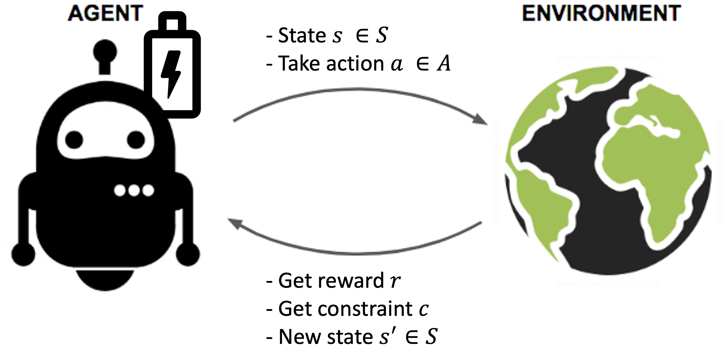
Based on an observation (also called state) from the environment, the agent selects an action. This action is executed in an environment resulting in a new state and a reward that evaluates the action. Given the new state, the feedback loop repeats.
In Reinforcement Learning, the world is modeled as a Markov Decision Process (MDP) and the goal is to select a policy \(\pi\) which maximizes an expected cumulative reward \(J^π\).
\(J^π\) can be taken to be the infinite horizon discounted total return as
\[J^\pi = \mathbb{E}_{s\sim\mu} \left[ \sum_{t=0}^T \gamma^t r(s_t, a_t) \right]\]where \(\gamma\) is the discount factor, and \(r(s_t,a_t)\) is the reward function.
However, the agents must obey safety constraints in many real-world applications while achieving the goal. We can introduce a constraint objective analogous to the reward objective. This objective is typically defined as the expected constraint value over N time steps \(J^π_C = \mathbb{E}_{s\sim\mu} \left[ C(s) \right]\). The method of aggregating individual constraints over time can vary, e.g., using the average or the maximum constraint value over N time steps or even a discounted sum.
In the example of the robot, the aim could be to prolong the motor life of the various robots while still enabling them to perform the task at hand. Thus we constrain the robot motors from using high torque values. Here, constraint C is defined as the average torque the agent has applied to each motor, and the penalty \(c(s, a)\) becomes the average amount of torque the agent decided to use at each time step.
We limit the allowable amount of torque applied to \(\alpha\).
The constrained MDP for our safe reinforcement learning problem is:
Constrained Policy Optimization
Constrained objectives are often solved using the Lagrange relaxation technique. With parameterized approaches such as Neural Networks, the objective is then to find the networks parameters \(\theta\) that maximize \(J^\pi_R\) subject to the constraint \(J^\pi_C \leq \alpha\) given the Lagrangian multiplier \(\lambda\):
\[\min_{\lambda}\max_{\theta} [J^{\pi_\theta}_R - \lambda (J^{\pi_\theta}_C - \alpha)]\]We now have our new global objective function that is subject to optimization!
What exactly does the Lagrangian do?
Intuitively, the Lagrangian multiplier \(\lambda\) determines how much weight is put onto the constraint. If \(\lambda\) is set to 0, the constraint is ignored, and the objective becomes the reward objective \(J^\pi_R\). If \(\lambda\) is set very high, the constraint is enforced very strictly, and the global objective function reduces to the constraint objective \(J^π_C\). Let’s look at a simple example to demonstrate the effect of the Lagrangian multiplier \(\lambda\). We’ll use the simple CartPole Gym environment. The reward in this environment is +1 for every step the pole was kept upright.
We can now add an example constraint to the environment. Let’s say we want to keep the cart in the left quarter of the x-axis. We, therefore, define the constraint value as the x-position of the cart and the upper bound \(\alpha\) as -2.
Let’s see how with different lambda values, the constraint is enforced.
The lower the lambda, the more the constraint is ignored. The higher the lambda, the more the constraint is enforced, and the main reward objective is ignored. At λ = 1,000,000 the cart shoots to the right to tilt the pole to the left but does so ignoring the following balancing act, which is observable at λ ∈ {10, 100}.
Tuning the \(\lambda\) through reward shaping is no easy feat. The Lagrangian is a scaling factor, i.e., if the constraint values are inherently larger than the reward values, we will need a substantially lower \(\lambda\) than when the constraint values are significantly smaller than the possible reward values. That means that the range of good lambda values is large and differs with every environment.
How can we learn an optimal Lagrangian?
Luckily, it is possible to view the Lagrangian as a learnable parameter and update it through gradient descent since the globally constrained optimization objective \(J^{\pi_{\theta}}\) is differentiable. In short, we can simply use the derivative of the objective function w.r.t \(\lambda\) and update the Lagrangian.
\[\frac{\partial J^{\pi_{\theta}}}{\partial \lambda} = -(J^{\pi_{\theta}}_C - \alpha)\] \[\lambda \gets max(\lambda - lr_{\lambda}(-(\mathbb{E}^{\pi_\theta}_{s\sim\mu} \left[C\right] - \alpha)), 0)\]Hereby \(lr_{\lambda}\) is the learning rate for the Lagrangian multiplier. The max function ensures that the Lagrangian multiplier is always positive.
Reward Constrained Policy Optimization
Actor-Critic based approaches such as PPO
How to integrate the constraint into the Actor-Critic approach?

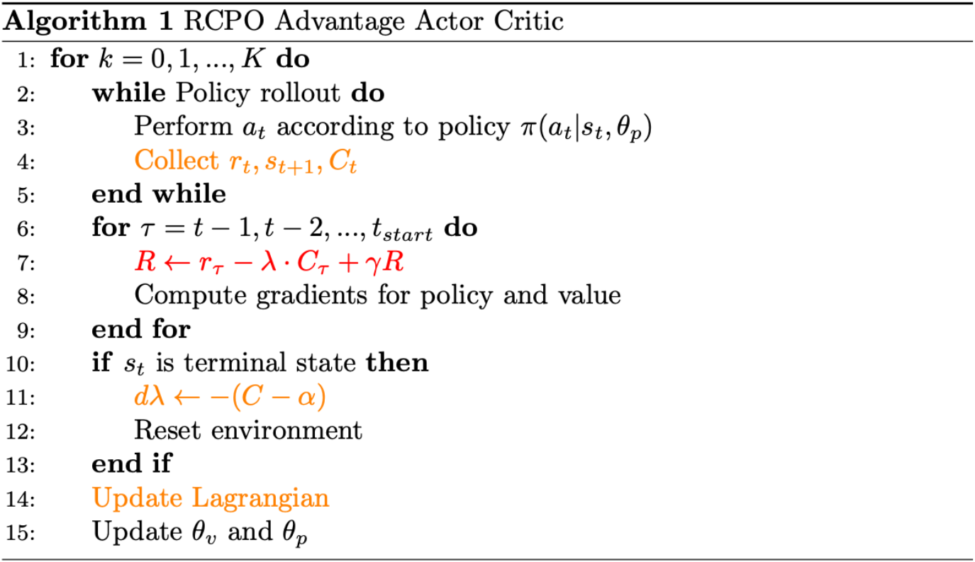
If we look at the RCPO algorithm illustrated above, we can see that implementing the constraint into the Actor-Critic approach is done in a few lines of code. First, we need to collect the constraint during the policy rollout. Then we can integrate the constraint values (the guiding penalty) into the reward during the computation of the policy and value gradients, as demonstrated in line 7.
This is done by formulating the constraint as the infinite horizon discounted total cost, similar to the usual returns of an MDP.
Now we can simply include the guiding penalty to the reward function via the Lagrange multiplier to arrive at the penalized reward function:
\[\hat{r} = r(s,a) - \lambda c(s,a)\]Finally, we can compute the gradient of the Lagrangian in line 11 and update \(\lambda\) in line 14 as discussed in the previous section and repeat the whole process for \(K\) times.
Implementation
To facilitate reproducibility, we integrated RCPO into the stable-baselines3
Integrating the guiding penalty
For the computation of returns with PPO, we use the Temporal Difference Error (TD estimate) and the Generalized Advantage Estimation (GAE) advantage.
To integrate the constraint into the reward function, we need to add the Lagrangian-scaled constraint value to the reward, as discussed in the RCPO section. This is done when computing the TD error estimate.
def compute_returns_and_advantages(
    self, last_values: th.Tensor, dones: np.ndarray
)
    # ...
    delta = (
        self.rewards[step]
        - self.constraint_lambda * self.constraints[step]
        + self.gamma * next_values * next_non_terminal
        -self.values[step]
    )
    # ...
The discussed integration of the constraint into the reward function is implemented into the computation of the advantages and returns. When the lambda parameter is set to 0, the constraint is ignored and the reward function is the same as in the original PPO implementation.
Additionally, it was necessary to extend the rollout buffer to collect the constraint values at each time step. To receive the constraint values, we customized the gym environments to return those in the info dictionary.
Updating the Lagrangian multiplier
Due to the fact that PPO (1) collects multiple episodes until the rollout buffers are full and (2) supports vectorized environments, the logic for collecting and aggregating the constraint values across the episodes and parallel environments is a bit more complex.
Nevertheless, we have chosen the aggregation method to be the average over all time steps in one complete episode and across all those episodes themselves, i.e., episodes that have reached a terminal state.
# lambda <- lambda - lr_lambda * -(C - alpha) = lambda + lr_lambda * (C - alpha)
d_constraint_lambda = self.C - self.constraint_lambda
self.rollout_buffer.constraint_lambda += (
    self.lr_constraint_lambda * d_constraint_lambda
)
self.rollout_buffer.constraint_lambda = np.maximum(
  self.rollout_buffer.constraint_lambda, 0
)
After aggregating the constraint values across the episodes and parallel environments into self.C, the Lagrangian is updated using gradient descent. The max function is used to ensure that the Lagrangian multiplier is always positive.
Experiments
As a proof-of-the-principle experiment, we reproduced the HalfCheetah task in OpenAI MuJoCo Gym from Tessler C. et al.
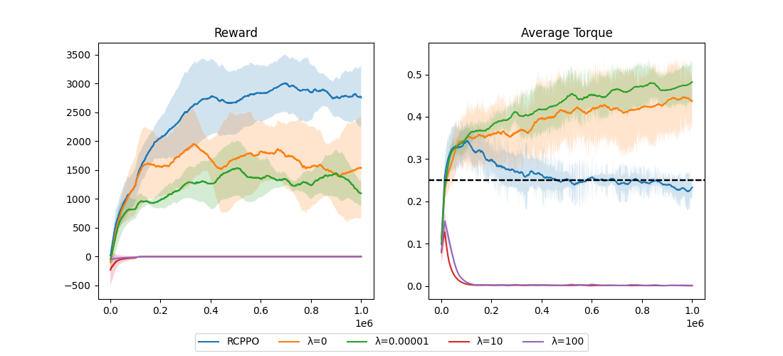
The results of the experiments are shown in the following figures. We kept (almost) all hyperparameters the same as in the original paper and let the agents train for \(1,000,000\) time steps.

The results demonstrate that the RCPPO trained an agent that successfully walked forward while respecting the safety constraint. We achieved comparable results to the original experiments in the paper.
Interestingly, low \(\lambda\) values seem to be less stable than higher \(\lambda\) values. The guiding penalty appears to enforce the constraint and improve the learning process overall. They limit the amount of torque the agent is allowed to apply, hinder the exploration of unsafe and poor-performing local minima and guide the policy to a safe and more optimal solution.
Nevertheless, the poor performance of the unconstrained agents may be due to the neural network architecture being relatively small (i.e., 2 layers of 64 hidden units).
Qualitative observations
Finally ,let’s see how our HalfCheetah agents walk under the To do so, we have recorded videos of the agents walking forward with different \(\lambda\) values. The results can be seen below.
We can again observe that the lower the lambda is, the more the constraint is ignored and the higher the lambda, the more the constraint is enforced and the main reward objective is ignored.
At λ ∈ {10, 100}, the robot applies 0 torque to ultimately oblige to the constraint ignoring the main reward objective to walk forward, which is observable at λ ∈ {RCPPO, 0, 0.00001}. With λ ∈ {0, 0.00001} the robot can walk forward, but it is visible that it moves its legs much quicker and more aggressively than the RCPPO agent. Furthermore, the RCPPO agent walks perfectly, whilst the other (moving) agents tumble over their own hecktick steps.
Discussion
Theoretical assumptions vs. empirical results
We had to select higher values for the Lagrangian multiplier than what were used in the original paper. In the paper, a \(\lambda\) value of 0.1 is already very high as it leads to a reward of \(-0.4\) and torque of \(0.1387\), whereas in our case a \(\lambda\) value of \(1.0\) leads to a reward of about \(1 500\) with an average torque of \(0.39\).
This affected the reward shaping process but also meant we had to increase the Lagrangian’s respective learning rate when training it as a parameter to grow quicker. As a result, \(lr_{\lambda}\) becomes larger than \(lr_{\pi}\), which ignores one of the assumptions made in the paper, yet leads to coherent results.
A possible reason for the slower and weaker impact of the constraint could be attributed to the clipping of the trust region. This technique ensures that the policy does not change too much between updates and prevents it from landing in a bad local minimum that it can not escape. This is done by clipping the policy update to a specific range. Therefore, even with “high” values of lambda w.r.t. the original paper, the policy will not change significantly to conform to the constraint.
Not only did we have to select a higher learning rate for the Lagrangian, but we also did not include different learning rates for the policy and the value function, ignoring the three times scales approach proposed in the original paper. Additionally, in the original paper the RCPPO algorithm updated their networks (actor and critic) after each episode. In our implementation, we need to fill the rollout buffer with potentially multiple episodes, thus reducing the frequency of network parameters and Lagrangian updates. Nevertheless, the PPO algorithm implements a parameter update loop of n epochs after each rollout, which to a degree counteracts the discussed lower update frequency of all parameters.
Conclusion
The results of the experiments show that the RCPO approach can learn a policy that can optimize the main reward objective while respecting the constraint.
Safe Reinforcement Learning is a critical area of research in the field of artificial intelligence, as it has the potential to shape the future of autonomous systems in a multitude of domains, ranging from robotics to finance.
The more complex systems become, the more difficult it is to ensure safety requirements, especially through simple reward shaping. An approach such as RCPO can ensure that the safety constraints are respected while enforcing them by only providing the constraint itself.