Underfitting and Regularization: Finding the Right Balance
In this blog post, we will go over the ICLR 2022 paper titled NETWORK AUGMENTATION FOR TINY DEEP LEARNING. This paper introduces a new training method for improving the performance of tiny neural networks. NetAug augments the network (reverse dropout), it puts the tiny model into larger models and encourages it to work as a sub-model of larger models to get extra supervision.
Goal of this blog post
Network Augmentation aka NetAug
Background
NetAug solely focuses on improving the performance of the tiny neural networks during inference, whilst optimizing their memory footprint to deploy them on edge devices. Tiny neural networks are usually inclined to underfit. Hence, the traditional training paradigms will not work for these small models because they fundamentally tackle the problem of overfitting and not overcome the underfitting issue. Several techniques in the recent time like data augmentation, pruning, dropout, knowledge distillation have been proposed to improve the generalizability of neural networks.
-
- Knowledge Distillation
- It is quite difficult to deploy and maintain an ensemble. However, previous research has shown that it is possible to learn a single cumbersome model that has the same performance as an ensemble. In most knowledge distillation methods there exist a large teacher model that transfers its knowledge as a learned mapping via training to a small student model with the teacher models output. There exists several techniques like self-distillation in which the teacher model trains itself continuously. Convectional KD methods try to optimise the objective function such that the loss function penalizes the difference between the student and teacher model.
- Knowledge Distillation
-
- Regularization
- Regularization is used to prevent overfitting of any ML model by reducing the variance, penalizing the model coefficients and complexity of the model. Regularization techniques are mainly composed of data augmentation one of the most simplest and conveninet ways to expand the size of the dataset such that it prevents overfitting issues that occur with a relatively small dataset. Dropout is also popularly applied while training models, in which at every iteration incoming and outgoing connections between certain nodes are randomly dropped based on a particular probability and the remaining neural network is trained normally.
- Regularization
-
- Tiny Deep learning
, , - Several challenges are paved while transitioning from conventional high end ML systems to low level clients, maintaining the accuracy of learning models, provide train-to-deploy facility in resource economical tiny edge devices, optimizing processing capacity. This method includes AutoML procedures for designing automatic techniques for architecturing apt neural netowrks for a given target hardware platform includes customised fast trained models,auto channel pruning methods and auto mixed precision quantization. The other approaches like AutoAugment methods automatically searches for improvised data augmentation within the network to prevent overfitting. There exists network slimming methods to reduce model size, decrease the run-time memory footprint and computing resource.
- Tiny Deep learning
-
- Network Augmentation
- This method was proposed to solve the problem of underfitting in tiny neural networks. This is done by augmenting the given model (referred to as base model) into a larger model and encourage it to work as a sub-model to get extra supervision in additoin to functioning independently. This will help in increasing the representation power of the base model because of the gradient flow from the larger model and it can be viewed equivalently as “reverse-dropout”.
- Network Augmentation
-
- Neural Architechture Search (NAS)
- This method was proposed to solve the problem of architecture optimization and weight optimization based on the underlying training data. NAS usually involves defining an architectural search space and then searching for the best architecture based on the performance on the validation set. Recent approaches include weight sharing, nested optimization and joint optimization during training. However, there are drawbacks in using these approaches because they are computationally expensive and suffer from coupling between architecture parameters and model weights. This will degrade the performance of the inherited weights.
- Neural Architechture Search (NAS)
Formulation of NetAug
The end goal of any ML model is to be able to minimize the loss function with the help of gradient descent. Since tiny neural network have a very small capacity the gradient descent is likely to get stuck in local minima. Instead of traditional regularization techniques which add noise to data and model, NetAug proposes a way to increase the capacity of the tiny model without changing its architecture for efficient deployment and inference on edge devices. This is done by augmenting the tiny model (referred to as base model) into a larger model and jointly training both the base model independently and also the augmented model so that the base model benefits from the extra supervision it receives from the augmented model. However, during inference only the base model is used.
To speed-up the training, a single largest augmented model is constructed by augmenting the width of the each layer of the base model using an augmentation factor \(r\). After building the largest augmented model, we construct other augmented models by selecting a subset of channels from the largest augmented model. NetAug proposes a hyper-parameter \(s\), named diversity factor, to control the number of augmented model configurations. We set the augmented widths to be linearly spaced between \(w\) and \(r \times w\). For instance, with \(r = 3\) and \(s = 2\), the possible widths would be \([w, 2w, 3w]\).
Pitfalls in NetAug
-
- Training the Generated Augmented Models
- NetAug randomly samples sub-models from the largest model by augmenting the width instead of depth, its highly important to ensure we speed up the training time and reduce the number of traning iterations for these generated sub-models thereby enhancing the training convergence and reaching optimization faster. We theoretically aim at aiding this by introducing a re-parametrisation technique during training that involves sharing and unsharing of weights to attain convergence much faster.
-
- Naive Loss Function
- NetAug computes loss in a very trivial form, i.e, by simply performing a weighted sum over the loss of the base model with that from the respective sampled augmented models. However, it was mentioned in the paper that sampling more than one sub-models from the largest augmented model in each training step is resulting in degradation of the base model’s performance. This can be attributed to the fact that simple weighted sum of losses from the base supervision and auxiliary supervision is causing the auxiliary supervision to shadow the base model. We propose different mixing strategies to circumvent this problem.
-
- Generating the Largest Augmented Model
- For a particular network, rather than tuning for just a single network hyperparameter (i.e., network, depth, width etc.), what if we instead tune all the closely relevant network hyperparameters for every augmented sub-model? To advocate this it’s sensible to compare the entire distribution of hyperparameter across the model. This can be tackled using NAS to find the best largest augmented model and then use it for auxiliary supervision of the base model.
Introducing NetAug with Relation Knowledge Distribution (RKD)
Knowledge distillation in learned models is constituted of:
-
- Individual Knowledge Distillation
- Outputs of individual samples represented by the teacher and student are matched.
-
- Relational Knowledge Distillation
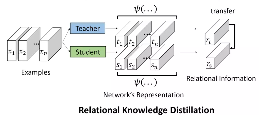
- Relation among examples represented by the teacher and student are matched. RKD is a generalization of convectional knowledge distillation that combines with NetAug to boost the performance due to its complementarity with conventional KD, that aims at transferring structural knowledge using mutual relations of data examples in the teacher’s output presentation rather than individual output themselves. Contrary to conventional approaches called as Individual KD (IKD) that transfers individual outputs of the teacher model \(f_T(\cdot)\) to the student model \(f_S(\cdot)\) point-wise, RKD transfers relations of the outputs structure-wise and computes a relational potential \(\psi\) for every \(n\)-tuple of data instance and transfers the relevant information through the potential from the teacher to the student models. In addition to knowledge represented in the output layers and the intermediate layers of a neural network, knowledge that captures the relationship between feature maps are also used to train a student model.
We specifically aim at training the teacher and student model in a online setting, in this online type of distillation training method both the teacher and the student model are trained together simultaneously.

Relational Knowledge distillation can be expressed as -
Given a teacher model \(\:T\:\) and a student model \(S\), we denote \(f_T(\cdot)\) and \(f_S(\cdot)\) as the functions of the teacher and the student, respectively, and \(\psi\) as a function extracting the relation, we have
where \(\mathcal{L}_{\text{RKD}}\) is the loss function, \(t_i = f_T(x_i)\) and \(s_i = f_S(x_i)\) and \(x_i \in \chi\) denotes the input data.
Loss Functions in RKD
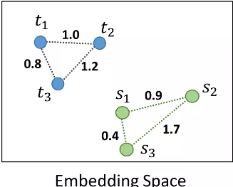
- Distance-wise distillation loss (pair)

This method is known as RKD-D. It transfers relative distance between points on embedding space. Mathematically, \(\begin{equation}\psi_{D}(t_i, t_j) = \frac{1}{\mu}\big\| t_i - t_j\big\|_2\end{equation}\) where \(\psi_d(\cdot, \cdot)\) denotes distance wise potential function \(\begin{equation}\mu = \frac{1}{|\chi^2|}\sum\limits_{(x_i, x_j) \in \chi^2} \big\| t_i - t_j\big\|_2\end{equation}\) \(\begin{equation}\boxed{\mathcal{L}_{\text{RKD-D}} = \sum \limits_{(x_i, x_j) \in \chi^2} l_\delta \big(\psi_D(t_i, t_j), \psi_D(s_i, s_j)\big)}\end{equation}\) where \(l_{\delta}\) denotes the Huber Los
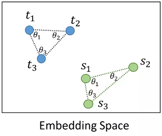
\[\begin{equation}l_\delta(x, y) = \begin{cases} \frac{1}{2} (x-y)^2\:\:\:\: \text{for } |x-y| \leq 1 \\ |x - y| - \frac{1}{2}\:\:\: \text{otherwise.} \end{cases}\end{equation}\]- Angle-wise distillation loss (triplet)

This method is known as RKD-A. RKD-A transfers angle formed by three points on embedding space. Mathematically, \(\begin{equation}\psi_{A}(t_i, t_j, t_k) = \cos \angle t_it_jt_k = \langle \boldsymbol{e}^{ij}, \boldsymbol{e}{jk}\rangle\end{equation}\) where \(\psi_A(\cdot, \cdot, \cdot)\) denotes angle wise potential function \(\begin{equation}\boldsymbol{e}^{ij} = \frac{t_i - t_j}{\big\|t_i - t_j\big\|_2}, \: \boldsymbol{e}^{jk} = \frac{t_k - t_j}{\big\|t_k - t_j\big\|_2}\end{equation}\)
\[\begin{equation}\boxed{\mathcal{L}_{\text{RKD-A}} = \sum\limits_{(x_i, x_j, x_k) \in \chi^3} l_\delta \big(\psi_A(t_i, t_j, t_k), \psi_A(s_i, s_j, s_k)\big)}\end{equation}\]Combining RKD with NetAug
We propose the following loss function to solve naive loss problem of NetAug
\[\begin{equation}\mathcal{L}_{\text{aug}} = \underbrace{\mathcal{L}(W_t)}_{\text{base supervision}} \:+\: \underbrace{\alpha_1 \mathcal{L}([W_t, W_1]) + \cdots + \alpha_i \mathcal{L}([W_t, W_i]) + \cdots}_{\text{auxiliary supervision, working as a sub-model of augmented models}} \:+\: \lambda_{\text{KD}}\,\underbrace{\mathbf{\mathcal{L}_{\text{RKD}}}}_{\text{relational knowledge distillation}}\label{eqn:loss_func}\end{equation}\]where \([W_t, W_i]\) represents an augmented model where \([W_t]\) represents the tiny neural network and \([W_i]\) contains weight of the sub-model sampled from the largest augmented model, \(\alpha\) is scaling hyper-parameter for combining loss from different augmented models and finally \(\lambda_{\text{KD}}\) is a tunable hyperparameter to balance RKD and NetAug.
NetAug Training with RKD
In NetAug, they train only one model for every epoch, training all the augmented models all once is not only computationally expensive but also impacts the performance. The proportion of the base supervision will decrease when we sample more augmented networks, which will make the training process biased toward augmented networks and shadows the base model.
To further enhance the auxiliary supervision, we propose to use RKD in an online setting i.e., the largest augmented model will act as a teacher and the base model will act as a student. Both the teacher and the student are trained simultaneously.
We train the both the base model and the augmented model via gradient descent based on the loss function \(\eqref{eqn:loss_func}\). The gradient update for the base model is then given by
\[\begin{equation}W^{n+1}_t = W^n_t - \eta \bigg(\frac{\partial \mathcal{L}(W^n_t)}{\partial W^n_t} + \alpha \frac{\partial \mathcal{L}([W^n_t, W^n_i])}{\partial W^n_t} + \lambda \frac{\partial \mathcal{L}_{\text{RKD}}([W^n_t, W^n_l])}{\partial W^n_t}\bigg)\end{equation}\]Similar update equations can be obtained for the largest augmented model and the sub-models as well.
Fasten Auxillary Model Training
We propose this method to solve the problem training the generated augmented models. Based on
Mathematical Formulation
Denote the neural model as consisting of \(L\) stacked structurally similar modules as \(\mathcal{M} = \{\mathcal{M}_i\}, \, i=1,\cdots, L\) and \(w = \{w_i\}, \, i=1,\cdots, L\) denote the corresponding weights. These weights are re-parametrized as
\[\begin{equation}w_i = \frac{1}{\sqrt{L}}w_0 + \tilde{w}_i, \:\:\:\: i=1,\cdots,L\end{equation}\]Here \(w_0\) represents the shared weights across all modules and is referred to as stem-direction and \(\tilde{w}_i\) represents the unshared weights across all modules and is referred to as branch-directions.
Training Strategy
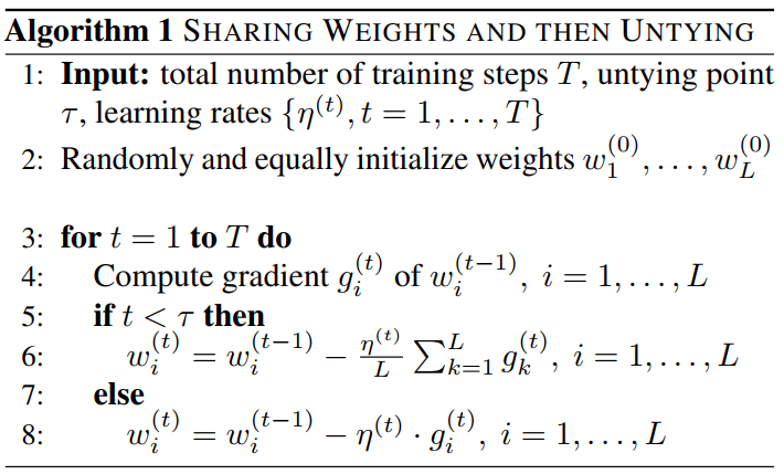
Denote \(T\) as the number of training steps, \(\eta\) as the step size and \(\alpha \in (0, 1)\) is a tunable hyper-paramter indicating the fraction of weight sharing steps. Then we train \(\mathcal{M}\) as follows:
- Sharing weights in early stage: For the first \(\tau = \alpha \cdot T\) steps, we update the shared weights \(w_0\) alone with gradient \(g_0\)
- Unsharing weights in later stage: For the next \(t \geq \alpha \cdot T\), we update only the unshared weights \(\tilde{w}_i\) with gradient \(\tilde{g}_i\)
The effective gradient updates for \(w_i\) can be found using chain rule as follows:
\[\begin{equation}g_0 = \frac{\partial \mathcal{L}}{\partial w_0} = \sum\limits_{i=1}^L \frac{\partial \mathcal{L}}{w_i}\,\frac{\partial w_i}{\partial w_0} = \frac{1}{\sqrt{L}}\sum\limits_{i=1}^L g_i \end{equation}\] \[\begin{equation}\tilde{g}_i = \frac{\partial \mathcal{L}}{\partial \tilde{w}_i} = \frac{\partial \mathcal{L}}{\partial w_i}\,\frac{\partial w_i}{\partial \tilde{w}_i} = g_i\end{equation}\]where \(g_i\) denotes the gradients of \(w_i\) and \(\mathcal{L}\) denotes the loss function.

Generating largest augmented model via Single Path One-Shot NAS
We propose this method to solve the problem of generating the largest augmented model. In NetAug, the largest augment model is generated randomly just based on the hyperparameters \(r\) and \(s\). Single Path One-Shot NAS with uniform sampling
-
Supernet weight Optimization : \(\begin{equation}W_{\mathcal{A}}=\mathop{\arg \min}_{W} \: \mathcal{L}_{\text{train}}\big(\mathcal{N}(\mathcal{A},W)\big)\end{equation}\)
The \(\mathcal{A}\) is the architecture search space represented as a directed acyclic graph which is encoded as a supernet \(\mathcal{N}(\mathcal{A}, W)\). During an SGD step in the above equation, each edge in the supernet graph is randomly dropped, using a dropout rate parameter. In this way, the co-adaptation of the node weights is reduced during training making the supernet training easier.
-
Architecture Search Optimization : \(\begin{equation}a^* = \mathop{\arg \max}_{a \in \mathcal{A}} \text{ ACC}_{\text{val}}\bigg(\mathcal{N}\big(a,W_{\mathcal{A}}(a)\big)\bigg)\end{equation}\)
During search, each sampled architecture a inherits its weights from \(W_{\mathcal{A}}\) as \(W_{\mathcal{A}}(a)\). The architecture weights are ready to use making the search very efficient and flexible. This type of sequential optimization works because, the accuracy of any architecture \(a\) on a validation set using inherited weight \(W_{\mathcal{A}}(a)\) (without extra fine tuning) is highly predictive for the accuracy of \(a\) that is fully trained. Hence we try to minimize the training loss even further for better performance, supernet weights \(W_{\mathcal{A}}\) such that all the architectures in the search space are optimized simultaneously.
where \(\Gamma(\mathcal{A})\) is the prior distribution of \(a \in \mathcal{A}\). This stochastic training of the supernet is helpful in better generalization of the optimized model and is also computationally efficient. To overcome the problem of weight coupling, the supernet \(\mathcal{N}(\mathcal{A},W)\) is chosen such that each architecture is a single path so that this realization is hyperparameter free as compared to traditional NAS approaches. The distribution \(\Gamma(\mathcal{A})\) is fixed apriori as a uniform distribution during our training and is not a learnable parameter.
Evaluation and Inference
Evaluation metric is the core for building any accurate machine learning model. We propose to implement the evaluation metrics precision@\(k\) ,recall@\(k\) and f1-score@\(k\) for the augmented sub-models sampled from largest augmented model and for the base model itself, where \(k\) represents the top k accuracy on the test set. These metrics will assist in evaluating the training procedure better than vanilla accuracy because we are trying to tackle the problem of underfitting, and an underfitted model is more likely to make the same prediction for every input and presence of class imbalance will lead to erroneous results.
Conclusion
The main conclusion of this blog post is to further refine tiny neural networks effectively without any loss in accuracy and prevent underfitting in them. The paper implements this in a unique way apart from the conventional techniques such as regularization, dropout and data augmentation. This blog adds to other techniques that are orthogonal to NetAug can be used combined with NetAug for improvised results.