Transformers Learn Faster by Taking Notes on the Fly
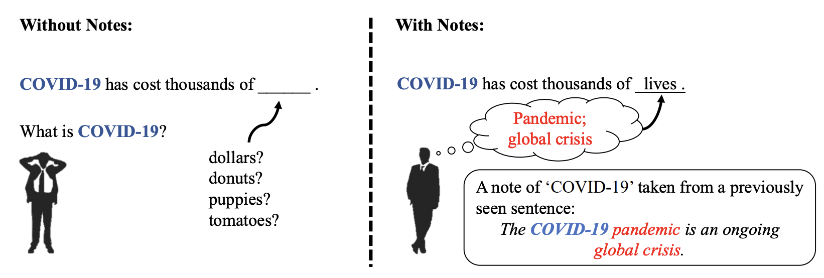
If your unsupervised pre-training is taking forever and you need a lightweight solution that will accelerate it, taking notes might be the method you are looking for! This method takes notes of the contextual information of the rare words and incorporates this information as a part of their embeddings on the fly! The solution is lightweight in the sense that it does not increase the inference time and it does not require an additional pass during training. The experiments demonstrate that this method reduces the pre-training time of large language models by up to 60%.
Introduction
Transformers, which were invented by Google in 2017
-
They are phenomenal in grasping the context of words within the bodies of text that they belong to.
-
They do not process the input sequences in order. Thus, their operations can easily be parallelized.
Equipped with these powerful features, transformers have excelled in unsupervised pre-training tasks, which is the driving force of several state-of-the-art models, such as BERT and GPT-3. In unsupervised pre-training, a large and diverse dataset is used to train the (baseline) model. If someone wishes to fine-tune the base model for a specific task, they can do so by training it with a relatively smaller, task-specific dataset.
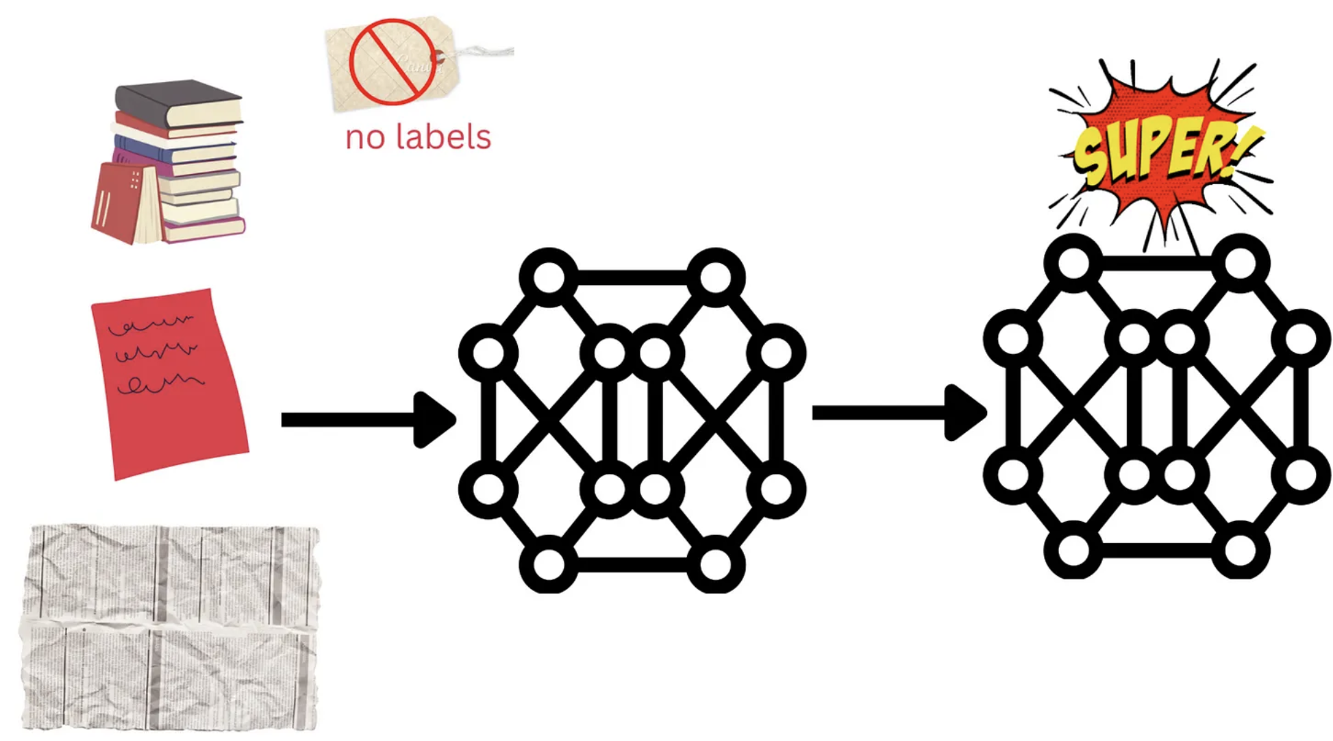
Generalization can be achieved with a sufficiently large model that is trained on sufficiently diverse and large data
Background
Transformers
Wu et al.
where \(pos\) is the position of the token in the sentence, \(d_{embed}\) is the embedding dimension of the model, and \(i\) refers to the dimension in the \(PE\) vector. Note that the positional embeddings do not depend on the meaning of the words, but only the position of them!
Self attention mechanism allows the model to relate words in a sentence through a set of learnable query \((Q)\), key \((K)\) and value \((V)\) vectors. The output of the attention function calculates a compatibility score for each pair of words in the sentence. Mathematically, self attention can be expressed as
\[\text{self-attention} (Q,K,V) = softmax(QK^T / \sqrt{(d_k)}),\]where \(d_k\) is the dimension of hidden representations. In order to improve the representational power of the model,
BERT is a masked language model which uses the transformer architecture. During training time, 15% of the words in the sentence are masked or replaced with a random word. The model learns to predict the words that are masked.
Word Distribution in Texts
The distribution of the words in a natural language corpora follow Zipf’s law
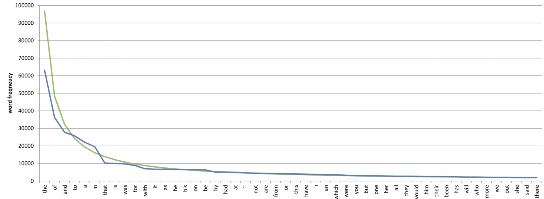
In other words, number of popular words are much less than of rare words, yet their frequency is much larger. This harms pretraining of LLMs because of the sparse and inaccurate optimization of neural networks, rare words are much likely to generate noisy and low-quality embeddings
Related Work
Pre-training of LLMs has become a burden in terms of training time and power consumption. Still, it is essential for almost every downstream task in NLP. This computational cost is addressed by several studies in terms of altering the model or utilizing the weight distribution of neural networks’ layers. Particularly,
The efficiency of pretraining LLMs has shown to be incresed, still the heavy-tailed distribution of words in natual language corpora is an obstacle in further development
It is shown that the frequency of words affect the embeddings. Additionally, most of the rare words’ embeddings are close to each other in embedding space indepent from its semantic information while the neighbors of frequent words are the ones that have similar meaning
Methodology
Because learning the embeddings of rare words is arduous, it takes a lot of training epochs for the model to make up for the resulting loss in quality. Thus, the authors propose keeping a third type of embedding (besides the word embeddings and positional embeddings), which is designed to retain additional information about the rare words. This embedding type can be considered as taking notes on the contextual information of these rare words as the training progresses, is also called the note dictionary, and is updated as the training progresses.
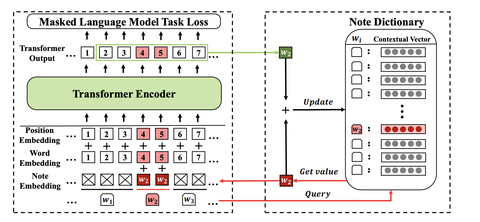
At this point, we assume that the text has already been pre-processed using Byte Pair Encoding (BPE
The first three steps are about initializing the required variables and determining the hyper-parameters of the scheme.
0a. Randomly initialize the note dictionary, \(NoteDict\).
0b. Determine a window size (\(2k\) as denoted in the paper), which corresponds to the number of surrounding tokens whose embedding will be included in the note.
0c. Determine a discount factor, \(\gamma\in (0,1)\). This will determine how much weight we give to each occurrence of the rare word and the corresponding contextual information.
Now, note taking begins!
1.For each word \(w\) in the training corpora, check if the word is a rare word or not. If it is rare, mark the index of the starting and ending sub-word tokens of the word with \(s\) and \(t\), respectively.
2.Compute the output of the transformer encoder on the input embeddings (positional+token+note embeddings). The output will be composed of \(d\)-dimensional vector per token. Call the output of the transformer encoder on position \(j\), \(c_j\in \mathbb{R}^d\).
3.Given a sequence of tokens \(x\) with word \(w\) in it, sum the \(d\)-dimensional input embedding vectors of all tokens located between indices \(s-k\) and \(t+k\) and divide this sum by \(2k+t-s\), namely, the number of tokens within that interval. The resulting vector is the note of \(w\) taken for sequence \(x\), \(Note(w,x)\). Mathematically, we have \(Note(w,x)=\dfrac{1}{2k+t-s}\sum_{j=s-k}^{t+k}c_j\).

4.To update the note embedding of w, NoteDict(w), take the exponential moving average of its previous value and Note(w,x) using the discount factor, namely, \(NoteDict(w)=(1-\gamma)NoteDict(w)+\gamma Note(w,x)\). This way, we can choose how much importance we assign to each occurrence of a rare word.
This process repeats until all of the sentences are processed this way. Note that, this can be achieved on the fly, as the model processes each sentence. Now that we have our notes neatly stored in \(NoteDict\), let us incorporate them into the training process! We again take the exponential moving average of the sum of the positional and token embeddings (the embedding used in the original transformer paper) with the corresponding \(NoteDict\) value using another parameter called \(\lambda\in(0,1)\). In particular, for every word \(w\) that occurs in both \(NoteDict\) and sequence \(x\), each location corresponding to the word \(w\) and its surrounding \(2k\) tokens is set to the weighted of the sum of the positional and token embeddings with the corresponding NoteDict value. Any other location is set to the sum of the token embeddings and positional embeddings only. The resulting vector will be the input to our model for the next step. Mathematically, for location \(i\in[d]\), which corresponds to (one of the) tokens of word \(w\) in the sequence, we have \(\text{input}_i= \begin{cases} (1-\lambda)(\text{p_embed}_i+\text{t_embed}_i)+\lambda\text{NoteDict}(w), & \text{w is a rare word} \\ \text{p_embed}_i+\text{t_embed}_i, &\text{otherwise} \\ \end{cases}\) where \(\text{p_embed}\) is positional embeddings, \(\text{t_embed}\) is token embeddings and \(\lambda\) (set to 0.5) is the hyperparameter specifying the weight of the notes when computing the embeddings.
Results
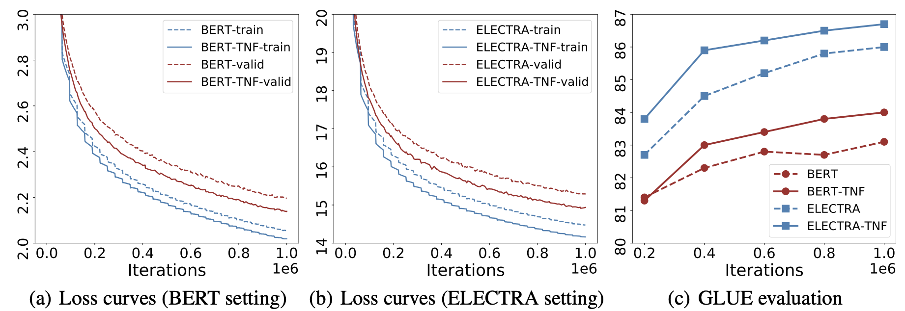
The experiments are conducted on BERT and ELECTRA models. The loss values of the pre-training runs with note taking descrease significantly faster than vanilla pre-training. Moreover, the models trained while taking notes achieve higher GLUE
Conclusion
The ever-increasing data sizes, enlarging models, and hardware resources are some of the major factors in the current success of LLMs. However, this also means immense power consumption and carbon emission. Because pre-training of LLMs is the most computationally intensive phase of a natural language task, efficient pre-training is the concern of this paper. Knowing that the heavy-tailed distribution of word frequencies in any natural language corpora may hinder the efficiency of pre-training, improving data utilization is crucial. Therefore, the authors propose a memory extension to the transformer architecture: “Taking Notes on the Fly”. TNF holds a dictionary where each key is a rare word. The values are the historical contextual information which is updated at each time the corresponding word is encountered. The dictionary is removed from the model during the inference phase. TNF reduces the training time by 60% without any reduction in the performance.